Start Here
Install the Server
Access the Server
Set Up a Folder & its Tools
Learn User Basics
Learn Admin Basics
Extend LabKey Server
Learn What's New in 9.1
9.1 Upgrade Tips
Learn What's New in 9.2
9.2 Upgrade Tips
Tutorials and Online Demos
Webinars and Videos
Roadmap for the Future
Administration
Installs and Upgrades
Before You Install
Install LabKey via Installer
Install LabKey Manually
Install Required Components
Configure the Web Application
Modify the Configuration File
Supported Tomcat Versions
Third-Party Components and Licenses
Manual install of caBIG™
Upgrade LabKey
Manual Upgrade
Upgrade PostgreSQL
Configure LDAP
Set Up MS Search Engines
Install the Enterprise Pipeline
Prerequisites for the Enterprise Pipeline
RAW to mzXML Converters
JMS Queue
Globus GRAM Server
Create a New Globus GRAM user
Configure LabKey Server to use the Enterprise Pipeline
Edit and Test Configuration
Using the Enterprise Pipeline
Configure the Conversion Service
Troubleshooting the Enterprise Pipeline
Install the Perl-Based MS2 Cluster Pipeline
Install the mzXML Conversion Service
Run the MS2 Cluster Pipeline
Example Setups and Configurations
Install CPAS on Linux
Example Installation of Flow Cytometry on Mac OSX
Configure FTP on Linux
Configure R on Linux
Configure the Virtual Frame Buffer on Linux
Set Up R
Set Up OpenSSO
Draft Material for OpenSSO
Customize "Look and Feel"
Troubleshooting
Projects and Folders
Create Project or Folder
Hidden Folders
Customize Folder
Reasons to Choose a "Custom"-Type Folder
Set Permissions
Manage Project Members
Navigate Folder Hierarchy
Move/Rename/Delete/Hide
Access Module Services
Add Web Parts
Manage Web Parts
Establish Terms of Use for Project
Security and Accounts
Site Administrator
Hide Admin Menus
User Accounts
Add Users
Manage Users
My Account
Anonymous Users
Security Groups
Global Groups
Project Groups
Site Groups
How Permissions Work
Permission Levels for Roles
Test Security Settings by Impersonating Users
Passwords
Authentication
Basic Authentication
Single Sign-On Overview
Admin Console
Site Settings
Look & Feel Settings
Web Site Theme
Additional Methods for Customizing Projects (DEPRECATED)
Navigation Element Customization (DEPRECATED)
Email Notification Customization
Backup and Maintenance
Administering the Site Down Servlet
Application & Module Inventory
Experiment
Xar Tutorial
XAR Tutorial Sample Files
Describing Experiments in CPAS
Xar.xml Basics
Describing Protocols
Describing LCMS2 Experiments
Overview of Life Sciences IDs
LSID Substitution Templates
Run Groups
Portal
Sub-Inventories
Application Inventory
Module Inventory
Web Part Inventory (Basic Wiki Version)
Web Part Inventory (Expanded Wiki Version)
Collaboration
Create a Collaboration Folder
Issues
Using the Issue Tracker
Administering the Issue Tracker
Messages
Using the Message Board
Administering the Message Board
Contacts
Wiki
Wiki Admin Guide
Wiki User Guide
Wiki Syntax Help
Advanced Wiki Syntax
Embed Live Content in Wikis
Web Part Configuration Properties
Wiki Attachment List
Discuss This
Study
Study Tutorial
Set up the Demo Study
Set up Datasets and Specimens
Sort and Filter Grid Views
Create a Chart
Create an R View
Create an R View with Cairo
Explore Specimens
Overview
Study Adminstrator Guide
Create a Study
Directly Create Study
Use Study Designer
Import/Export/Reload a Study
Study Import/Export Formats
Manage a Study
Manage Datasets
Manage Visits
Manage Labs and Sites
Manage Cohorts
Manage Study Security
Configure Permissions for Reports & Views
Matrix of Dataset- and Folder-Level Permissions
Manage Views
Define and Map Visits
Advice on Defining Visits
Manually Create and Map Visits
Create a Visit
Edit Visits
Map Visits
Identify Visit Dates
Import Visits and Visit Map
Create and Populate Datasets
Direct Import Pathway
Create a Single Dataset
Create a Single Dataset and Schema
Create Multiple Datasets and Schemas
Dataset Properties
Dataset Schema
Schema Field Properties
Pre-Defined Schema Properties
Date and Number Formats
Import Data Records
Import via Copy/Paste
Import From a Dataset Archive
Create Pipeline Configuration File
Assay Publication Pathway
Manage Your New Dataset
Set Up, Design & Copy Assays
Manage Specimens
Import a Specimen Archive
Import Specimens Via Cut/Paste
Set Up Specimen Request Tracking
Approve Specimen Requests
Create Reports And Views
Advanced Views
The Enrollment View
Workbook Reports
Annotated Study Schema
Study User Guide
Site Navigation
Study Navigation
The Study Navigator
Selecting, Sorting & Filtering
Reports and Views
Cohorts
Assays
Dataset Import & Export
Dataset Import
Dataset Export
Specimens
Specimen Shopping Cart
Specimen Reports
Wiki User Guide
Accounts and Permissions
Password Reset & Security
Permissions
Your Display Name
Proteomics
Get Started With CPAS
Explore the MS2 Dashboard
Upload MS2 Data Via the Pipeline
Set Up MS2 Search Engines
Set Up Mascot
Set Up Sequest
Install SequestQueue
Set the LabKey Pipeline Root
Search and Process MS2 Data
Configure Common Parameters
Configure X! Tandem Parameters
Configure Mascot Parameters
Configure Sequest Parameters
Sequest Parameters
MzXML2Search Parameters
Examples of Commonly Modified Parameters
Working with MS2 Runs
Viewing an MS2 Run
Customizing Display Columns
Peptide Columns
Protein Columns
Viewing Peptide Spectra
Viewing Protein Details
Viewing Gene Ontology Information
Comparing MS2 Runs
Exporting MS2 Runs
Protein Search
Peptide Search
Loading Public Protein Annotation Files
Using Custom Protein Annotations
Using ProteinProphet
Using Quantitation Tools
Experimental Annotations for MS2 Runs
Exploratory Features
caBIG™-certified Remote Access API to LabKey/CPAS
Spectra Counts
Label-Free Quantitation
MS1
MS1 Pipelines
CPAS Team
Flow Cytometry
LabKey Flow Overview
Flow Team Members
Tutorial: Import a FlowJo Workspace
Install LabKey Server and Obtain Demo Data
Create a Flow Project
Set Up the Data Pipeline and FTP
Place Files on Server
Import a FlowJo Workspace and Analysis
Customize Your View
Examine Graphs
Examine Well Details
Finalize a Dataset View and Export
Tutorial: Perform a LabKey Analysis
Create Custom Flow Queries
Locate Data Columns of Interest
Add Statistics to FCS Queries
Calculate Suites of Statistics for Every Well
Flow Module Schema
Add Sample Descriptions
Assays
Assay Administrator Guide
Set Up Folder For Assays
Design a New Assay
Property Fields
General Properties
ELISpot Properties
Luminex Properties
Microarray Properties
NAb Properties
Edit Plate Templates
Copy Assay Data To Study
Copy-To-Study History
Tutorial: Import Microarray Data
Install LabKey Server
Create a Microarray Project
Set Up the Data Pipeline and FTP
Assay User Guide
Import Assay Runs
Import General Assays
Import ELISpot Runs
Import Luminex Runs
Luminex Conversions
Import Microarray Runs
Import NAb Runs
Work With Assay Data
Data and Views
Dataset Grid Views
Participant Views
Selecting, Sorting & Filtering
Select Data
Sort Data
Filter Data
Custom Grid Views
Create Custom Grid Views
Select and Order Columns
Example: Create a "Joined View" from Multiple Datasets
Pre-Define Filters and Sorts
Save and View Custom Views
Reports and Views
R Views
The R View Builder
Author Your First Script
Upload a Sample Dataset
Access Your Dataset
Load Packages
Determine Available Graphing Functions
Graphics File Formats
Use Input/Output Syntax
Work with Saved R Views
Display R View on Portal
Create Advanced Scripts
Means, Regressions and Multi-Panel Plots
Basic Lattice Plots
Participant Charts
User-Defined Functions
R Tutorial Video for v8.1
FAQs for LabKey R
Chart Views
Crosstab Views
Static Reports
Manage Views
Custom SQL Queries
Create a Custom Query
Use the Source Editor
Use the Query Designer
Review Metadata in SQL Source Editor
Display a Query
Add a Calculated Column to a Query
Use GROUP BY and JOIN
Use Cross-Folder Queries
LabKey SQL Reference
Metadata XML
Lists & External Schemas
Lists
External Schemas
Search
Files
File Upload and Sharing
Set Up File Sharing
Use File Sharing
Pipeline
Set the LabKey Pipeline Root
Set Up the FTP Server
Upload Pipeline Files via FTP
BioTrue
APIs
Tutorial Video: Building Views and Custom User Interfaces
Client-Side APIs
JavaScript API
Tutorial: JavaScript API
Reagent Request Form
Reagent Request Confirmation Page
Summary Report for Reagent Managers
Licensing for the Ext API
Generate JavaScript
Example: Charts
Generate JSDoc
JavaScript Class List
Java API
Java Class List
R API
SAS API
Setup Steps for SAS
Configure SAS Access From LabKey Server
SAS Macros
SAS Security
SAS Demos
Server-Side APIs
Examples: Controller Actions
Example: Access APIs from Perl
How To Find schemaName, queryName & viewName
Web Part Configuration Properties
Implementing API Actions
Programmatic Quality Control
Using Java for Programmatic QC Scripts
Developer Documentation
Recommended Skill Set
Setting up a Development Machine
Notes on Setting up a Mac for LabKey Development
Machine Security
Enlisting in the Version Control Project
Source Code
Confidential Data
Development Cycle
Project Process
Release Schedule
Issue Tracking
Submitting Contributions
Checking Into the Source Project
Developer Email List
Wiki Documentation Tools
The LabKey Ontology & Query Services
Building Modules
Third-party Modules
Module Architecture
Simplified Modules
Queries, Views and Reports in Modules
Assays defined in Modules
Getting Started with the Demo Module
Creating a New Module
Deprecated Components
The LabKey Server Container
CSS Design Guidelines
Creating Views
Maintaining the Module's Database Schema
Integrating with the Pipeline Module
Integrating with the Experiment Module
GWT Integration
GWT Remote Services
UI Design Patterns
Feature Owners
LabKey Server and the Firebug add-on for Firefox
Start Here
Get Started With LabKey Server 9.1
- Administrators + Potential Adopters
- Users
- Developers
Version 9.1 Improvements
Training Materials
Still Have Questions?
- Search the documentation. Use the Search box in the upper right corner of this page.
- Search the community forums. Each forum has a search box on its upper right side.
- Obtain commercial support. LabKey Corporation provides consulting services to users who need assistance installing, enhancing and maintaining the LabKey Server platform in a production setting. Email info@labkey.com for further information.
- Review documentation archive. See Documentation for LabKey Versions 1.1-8.3
Future Directions for LabKey Server
Install the Server
This section explains how to install or upgrade LabKey Server.
Topics:
Access the Server
Log InMost LabKey projects are secured to protect the data they contain, so you will want to log in to access your projects. Depending on how LabKey is set up for your organization, you may be able to log in using your network user name and password, or you have have to request a LabKey account. If you're not sure, ask your administrator. He or she can create an account for you if you don't already have one, and also grant you project permissions as needed.
Once you've logged in, you can edit your account information by clicking on the My Account link in the upper right corner of any page.
Supported Browsers
LabKey is a web application that runs in your web browser. To access LabKey, you must use a web browser that LabKey supports.
- On Windows, you can use either Microsoft Internet Explorer or Mozilla Firefox.
- On Unix-based systems, use Firefox. The older Mozilla browser may also work, but it is not technically supported for use with LabKey.
- On the Macintosh, you must use Firefox to access LabKey. Other popular Mac browsers like Safari and Internet Explorer have serious problems with JavaScript, which is required for some key features of LabKey.
Set Up a Folder & its Tools
Learn User Basics
Prerequisites: Before you use LabKey Server, your Admin must
Install your server and
Set up your workspace.
Basic Activities
Specialized Activities
Read more about the
LabKey Applications you expect to use.
Explore
LabKey Modules. LabKey Modules can be added to LabKey Applications to extend their functionality. A few of the modules you may use:
Advanced Activities
Learn Admin Basics
Overview
[Community Forum]
Administrative features provided by LabKey Server include:
- Project organization, using a familiar folder hierarchy
- Role-based security and user authentication
- Dynamic web site management
- Backup and maintenance tools
Documentation Topics
Set Up Your Server
Maintain Your Server
Extend LabKey Server
Learn What's New in 9.1
Version 9.1 represents a important step forward in the ongoing evolution of the open source LabKey Server. Enhancements in this release are designed to:
- Support leading medical research institutions using the system as as a data integration platform to reduce the time it takes for laboratory discoveries to become treatments for patients
- Provide rapid to deploy software infrastructure for communities pursing collaborative clinical research efforts
- Deliver a secure data repository for managing and sharing laboratory data with colleagues, such as for proteomics, microarray, flow cytometry or other assay-based data.
New capabilities introduced in this release are summarized below.
For a full query listing all improvements made in 9.1, see:
Items Completed in 9.1. Refer to
9.1 Upgrade Tips to work around minor behavior changes associated with upgrading from v8.3 to v9.1.
Download LabKey Server v 9.1.
Quality Control
- Field-level quality control. Data managers can now set and display the quality control (QC) status of individual data fields. Data coming in via text files can contain the special symbols Q and N in any column that has been set to allow quality control markers. “Q” indicates a QC has been applied to the field, “N” indicates the data will not be provided (even if it was officially required).
- Programmatic quality control for uploaded data. Programmatic quality control scripts (written in R, Perl, or another language of the developer's choice) can now be run at data upload time. This allows a lab to perform arbitrary quality validation prior bringing data into the database, ensuring that all uploaded data meets certain initial quality criteria. Note that non-programmatic quality control remains available -- assay designs can be configured to perform basic checks for data types, required values, regular expressions, and ranges in uploaded data.
- Default values for fields in assays, lists and datasets. Dataset schemas can now be set up to automatically supply default values when imported data tables have missing values. Each default value can be the last value entered, a fixed value or an editable default.
- Display of assay status. Assay working folders now clearly display how many samples/runs have been processed for each study.
- Improved study integration. Study folders provide links to view source assay data and designs, as well as links to directly upload data via appropriate assay pipelines.
- Hiding of unnecessary "General Purpose" assay details. Previously, data for this type of assay had a [details] link displayed in the copied dataset. This link is now suppressed because no additional information is available in this case.
- Easier data upload. Previously, in order to add data to an assay, a user needed to know the destination folder. Now users are presented with a list of appropriate folders directly from the upload button either in the assay runs list or from the dataset.
- Improved copy to study process. It is now easier to find and fix incorrect run data when copying data to a study. Improvements:
- Bad runs can now be skipped.
- The run details page now provides a link so that run data can be examined.
- There is now an option to re-run an assay run, pre-populating all fields, including the data file, with the previous run. On successful import, the previous run will be deleted.
- Protein Search Allows Peptide Filtering. When performing a protein search, you can now filter to show only proteins groups that have a peptide that meets a PeptideProphet probability cutoff, or specify an arbitrarily complex peptide filter.
- Auto-derivation of samples during sample set import. Automated creation of derivation history for newly imported samples eases tracking of sample associations and history. Sample sets now support an optional column that provides parent sample information. At import time, the parent samples listed in that column are identified within LabKey Server and associations between samples are created automatically.
- Microarray bulk upload.
- When importing MageML files into LabKey Server, users can now include a TSV file that supplies run-level metadata about the runs that produced the files. This allows users to reuse the TSV metadata instead of manually re-entering it.
- The upload process leverages the Data Pipeline to operate on a single directory at a time, which may contain many different MageML files. LabKey Server automatically matches MageML files to the correct metadata based on barcode value.
- An Excel template is provided for each assay design to make it easier to fill out the necessary information.
- Microarray copy-to-study. Microarray assay data can now be copied to studies, where it will appear up as an assay-backed dataset.
- Support for saving state within an assay batch/run upload. Previously, once you started upload of assay data, you had to finish at one point in time. Now you can start by uploading an assay batch, then upload the run data later.
- NAb improvements:
- Auto-complete during NAb upload. This is available for specimen, visit, and participant IDs.
- Re-run of NAb runs. After you have uploaded a NAb run and you wish to make an edit, you can redo the upload process with all the information already pre-filled, ready for editing.
- Specimen shopping cart. When compiling a specimen request, you can now perform a specimen search once, then build a specimen request from items listed in that search. You can add individual vials one-at-a-time using the "shopping cart" icon next to each vial. Alternatively, you can add several vials at once using the checkboxes next to each vial and the actions provided by the "Request Options" drop-down menu. After adding vials to a request of your choice, you return to your specimen search so that you can add more.
- Auditing for specimen comments. Specimen comments are now logged, so they can be audited.
- Specimen reports can now be based on filtered vial views. This increases the power of reporting features.
- Enhanced interface for managing views. The same interface is now used to manage views within a study and outside of a study.
- Container filters for grid views. You can now choose whether the list of "Views" for a data grid includes views created within the current folder or both the current folder and subfolders.
- Ability to clear individual columns from sorts and filters for grid views. The "Clear Sort" and "Clear Filter" menu items area available in the sort/filter drop-down menu available when you click on a grid view column header. For example, the "Clear Sort" menu item is enabled when the given column is included in the current sort. Selecting that item will remove just that column from the list of sorted columns, leaving the others intact.
- More detailed information for the "Remember current filter" choice on the Customize View page. When you customize a grid view that already contains sorts and filters, these sorts and filters can be retained with that custom view, along with any sorts and filters added during customization. The UI now explicitly lists the pre-existing sorts and filters that can be retained.
- Stand-alone R views. You do not need to associate every R view with a particular grid view. R views can be created independently of a particular dataset through the "Manage Views" page.
- Improved identification of views displayed in the Reports web part. The Reports web part now can accept string-based form of report ID (in addition to normal integer report ID) so that you can refer to a report defined within a module.
- Ability to download a single FCS file. A download link is now available on the FCS File Details page.
- New Documentation: Demo, Tutorial and additional Documentation
- Richer filter UI for "background column and value." Available in the ICS Metadata editor. This provides support for "IN" and multiple clauses. Example: Stim IN ('Neg Cont', 'negctrl') AND CD4_Count > 10000 AND CD8_Count > 10000
- Performance improvements. Allow loading larger FlowJo workspaces than previously possible.
- UI improvements for FlowJo import. Simplify repeated uploading of FlowJo workspaces.
- New SAS Client API. The LabKey Client API Library for SAS makes it easy for SAS users to load live data from a LabKey Server into a native SAS dataset for analysis, provided they have permissions to read those data. It also enables SAS users to insert, update, and delete records stored on a LabKey Server, provided they have appropriate permissions to do so. All requests to the LabKey Server are performed under the user's account profile, with all proper security enforced on the server. User credentials are obtained from a separate location than the running SAS program so that SAS programs can be shared without compromising security.
- Additions to the Java, JavaScript, R and SAS Client Libraries:
- Additions to the Javascript API:
- Callback to indicate that a web part has loaded. Provides a callback after a LABKEY.WebPart has finished rendering.
- Information on the current user (LABKEY.user). The LABKEY.Security.currentUser API exposes limited information on the current user.
- API/Ext-based management of specimen requests. See: LABKEY.Specimen.
- Sorting and filtering for NAb run data retrieved via the LabKey Client APIs. For further information, see: LABKEY.Assay#getNAbRuns
- Ability to export tables generated through the client API to Excel. This API takes a JavaScript object in the same format as that returned from the Excel->JSON call and pops up a download dialog on the client. See LABKEY.Utils#convertToExcel.
- Improvements to the Ext grid.
- Quality control information available.
- Performance improvements for lookup columns.
- Documentation for R Client API. Available here on CRAN.
- File-based modules. File-based modules provide a simplified way to include R reports, custom queries, custom query views, HTML views, and web parts in your modules. You can now specify a custom query view definition in a file in a module and it will appear alongside the other grid views for the given schema/query. These resources can be included either in a simple module with no Java code whatsoever, or in Java-based modules. They can be delivered as a unit that can be easily added to an existing LabKey Server installation. Documentation: Overview of Simplified Modules and Queries, Views and Reports in Modules.
- File-based assays. A developer can now create a new assay type with a custom schema and custom views without having to be a Java developer. A file-based assay consists of an assay config file, a set of domain descriptions, and view html files. The assay is added to a module by placing it in an assay directory at the top-level of the module. For information on the applicable API, see: LABKEY.Experiment#saveBatch.
- Support for additional SQL functions:
- UNION and UNION ALL
- BETWEEN
- TIMESTAMPDIFF
- Cross-container queries. You can identify the folder containing the data of interest during specification of the schema. Example: Project."studies/001/".study.demographics.
- Query renaming. You can now change the name of a query from the schema listing page via the “Edit Properties” link.
- Comments. Comments that use the standard SQL syntax ("--") can be included in queries.
- Metadata editor for built-in tables. This editor allows customization of the pre-defined tables and queries provided by LabKey Server. Users can change number or date formats, add lookups to join to other data (or query results), and change the names and description of columns. The metadata editor shows the metadata associated with a table of interest and allows users to override default values. Edits are saved in the same XML format used to describe custom queries.
- Version comparison tool for wiki pages. Differences between older and newer versions of wiki pages can now be easily visualized through the "History"->"Compare Versioned Content"->"Compare With" pathway.
- Attachments can now be downloaded from the "Edit" page. Also, if an attachment is an image, clicking on it displays it in a new browser tab.
- Tomcat 5.5.27 is now supported.
- Upgrade to PostgresSQL 8.3 is now strongly encouraged. For anyone running PostgreSQL 8.2.x or earlier, you will now see a yellow warning message in the header when logged in as a system admin. Upgrade to PostgreSQL 8.3 to eliminate the message. The message can also be hidden. Upgrade documentation.
9.1 Upgrade Tips
PostgreSQL 8.3 Upgrade Tip for Custom SQL Queries
Problem. After upgrading to PostgreSQL 8.3, some custom SQL queries may generate errors instead of running. An example of an error message you might observe:
Query 'Physical Exam Query' has errors
java.sql.SQLException: ERROR: operator does not exist: character varying = integer
Solutions: Two Options.
1. Use the Query Designer. If your query is simple enough for viewing in the Query Designer:
- View your query in the Query Designer.
- Save your query. The Query Designer will make the adjustments necessary for compatibility with PostgreSQL 8.3 automatically.
- Your query will now run instead of generating an error message.
2. Use the Source Editor. If your query is too complicated for viewing in the Query Designer:
- Open it in the Source Editor.
- In the query editor, add single quotes around numbers so that they will be saved appropriately. For example, change
WHERE "Physical Exam".ParticipantId.ParticipantId=249318596
to:
WHERE "Physical Exam".ParticipantId.ParticipantId='249318596'
- Your query will now run instead of generating an error message.
Cause. As of LabKey Server v9.1, the Query Designer uses column types in deciding how to save comparison values. In versions of LabKey Server pre-dating v9.1, an entry such as 1234 became 1234 regardless of whether the column type was string or numeric. In LabKey Server v9.1, the Query Designer saves 1234 as '1234' if appropriate. Older queries need to be resaved or edited manually to make this change occur.
Learn What's New in 9.2
Overview
LabKey Server v 9.2 has not yet been released. This feature list provides a preview of the release.
Version 9.2 represents a important step forward in the ongoing evolution of the open source LabKey Server. Enhancements in this release are designed to:
- Support leading medical research institutions using the system as as a data integration platform to reduce the time it takes for laboratory discoveries to become treatments for patients
- Provide rapid to deploy software infrastructure for communities pursing collaborative clinical research efforts
- Deliver a secure data repository for managing and sharing laboratory data with colleagues, such as for proteomics, microarray, flow cytometry or other assay-based data.
New capabilities introduced in this release are summarized below.
For an exhaustive list of all improvements made in 9.2, see:
Items Completed in 9.2. Refer to the
9.2 Upgrade Tips to quickly identify behavioral changes associated with upgrading from v9.1 to v9.2.
After 9.2 is released: Download LabKey Server v 9.2.
User administration and security
Finer-grained permissions settings for administrators
- Tighter security. Admins can now receive permissions tightly tailored to the subset of admin functions that they will perform. This allows site admins to strengthen security by reducing the number of people who possess broad admin rights. For example, "Specimen Requesters" can receive sufficient permissions to request specimens without being granted folder administration privileges.
- New roles. LabKey Server v9.2 includes four entirely new roles: "Site Admin," "Assay Designer," "Specimen Coordinator" and "Specimen Requester." This spreadsheet shows a full list of the new admin roles and the permissions they hold. It also shows roles that may be added in future releases of LabKey Server.
Improved permissions management UI
- Brief list of roles instead of long list of groups. Previously, the permissions management interface displayed a list of groups and allowed each group to be assigned a role. This list became hard to manage when the list of groups grew long. Now security roles are listed instead of groups, so the list is brief. Groups can be assigned to these listed roles or moved between roles.
- Rapid access to users, groups and permission settings. Clicking on a group or user brings up a floating window that shows the assigned roles of that group or user across all folders. You can also view the members of multiple groups by switching to the groups tab.
Assignment of individual users to roles
- Now individual users, not just groups, can be assigned to security roles. This allows admins to avoid creating groups with single members in order to customize permissions.
Site Users list is a grid view
- This allows customization and export of the view.
Custom permission reporting
- Administrators can create custom lists to store metadata about groups by joining a list with groups data. Any number of fields can be added to information about a each user or group. These lists can be joined to:
- Built in information about the user (name, email etc)
- Built in information about the group (group, group members)
- The results can also be combined with built-in information about roles assigned to each user & group in each container. From this information a variety of reports can be created, including group membership for every user and permissions for every group in every container.
- These reports can be generated on the client and exported as Excel Spreadsheets
Improved UI for Deleting, Deactivating and Re-activating Users
- Deactivate/Re-Activate buttons are now on the user details page as well as the user list. When clicked on the user list, a confirmation page is shown listing all the selected users (users that are already activate/inactive are filtered out if action is deactivate/re-activate).
- Clicking Delete on the user list now takes you to a confirmation page much like the deactivate/re-activate users command. If at least one of the selected users is active, it will also include a note and button that encourages the admin to deactivate the user(s) rather than permanently delete them.
Study
Study export, import and reload
- Studies can be reloaded onto the same server or onto a different LabKey Server. This makes it easy to transfer a study from a staging environment to a live LabKey platform.
- You can populate a brand new study with the exported contents of an existing study. For similar groups of studies, this helps you leverage your study setup efforts.
- Studies can be set up to reloaded data from a data depot nightly. This allows regular transfer of updates from a remote, master database to a local LabKey Server. It keeps the local server up-to-date with the master database automatically.
Customizable "Missing Value" indicators
- Field-Level Missing Value (MV) Indicators allow individual data fields to be flagged. Previously, only two MV values were allowed (N and Q). Administrators can now customize which MV values are available. A site administrator can customize the MV values at the site level and project administrators can customize the MV values at the folder level. If no custom MV values are set for a folder, they will be inherited from their parent folder. If no custom values are set in any parent folders, then the MV values will be read from the server configuration.
- MV value customization consists of creating or deleting MV values, plus editing their descriptions.
- A new API allows programmatic configuration of MV values for a folder. This allows study import/export to include MV values in its data and metadata.
"Missing Value" user interface improvements
- MV values are now displayed with a pop-up and a MV indicator on an item’s detail page.
- When inserting or updating an item with a MV-enabled field, possible MV values are now offered in a drop-down, along with the ability to set a raw value for the field. Currently a user is only able to specify one or the other on the update page.
Specimens
Import of specimen data allowed before completion of quality control (QC)
- Specimen import is now more lenient in the conflicts it allows in imported specimen data. Previously, import of the entire specimen archive was disallowed if conflicts were detected between transaction records for any individual vial. In 9.2, all fields with conflicts between vials are marked "NULL" and the upload is allowed to complete.
- Use a saved, custom view that filters for vials with the "Quality Control Flag" marked "True" in order to identify and manage vials that imported with conflicts.
Visual flagging of all questionable vials and primary specimens
- Vial events with conflicting information are flagged. Conflicts are differentiated by the presence of an "unknown" value for the conflicting columns, plus color highlighting. For example, you would see a flag when an imported specimen's globalUniqueID is associated with more than one primary type, as could occur if a clinic and repository entered different vial information pre- and post-shipment.
- Vial events that indicate a single vial is simultaneously at multiple locations are flagged. This can occur in normal operations when an information feed from a single location is delayed, but in other cases may indicate an erroneous or reused globalUniqueID on a vial.
- Vials or primary specimens that meet user-specified protocol-specific criteria are flagged. Examples of QC problems that could be detected with this method include:
- A saliva specimen present in a protocol that only collects blood (indicating a possibly incorrect protocol or primary type).
- Primary specimen aliquoted into an unexpectedly large number of vials, based on protocol expectations for specimen volume (indicating a possibly incorrect participantID, visit, or type for one or more subset of vials).
Built-in report for mismatched specimens.
- The new "specimencheck" module identifies mismatched specimens and displays them in a grid view. It identifies specimens whose participantID, sequenceNum and/or visit dates fail to match, then produces a report that can be used to perform quality control on these specimens. For developers, the "specimencheck" module also provides an example of a simple file-based module.
Manual addition/removal of QC flags
- This allows specimen managers to indicate that a particular quality control problem has been investigated and resolved without modification of the underlying specimen data.
- A specimen manager can also manually flag vials as questionable even if they do not meet any of the previously defined criteria.
- Records of manual flagging/unflagging are preserved over specimen imports, in the same manner as specimen comments.
Blank columns eliminated from Excel specimen reports
- When exported to Excel, individual worksheets of specimen reports may include blank columns. This is due to the fact that columns are included for all visits that have specimens of any kind, rather than for just those visits with specimens matching the current worksheet’s filter. Exported Excel files now display a minimal set of visit columns per report worksheet.
Additional vial count columns available in vial views
- Additional columns can be optionally presented in vial view and exported via Excel. These include the number of sibling vials currently available, locked in requests, currently at a repository and expected to become available, plus the total number of sibling vials.
- These columns are available via the ‘customize view’ user interface, so different named/saved views can be created. The built-in ability to save views per user enables specimen coordinators to see in-depth detail on available counts, while optionally presenting other users with a more minimal set of information.
Performance
- Faster loading of specimen queries. Please review the 9.2 Upgrade Tips to determine whether any of your queries will need to be updated to work with the refactored specimen tables.
Specimen report improvements
- New filter options are available for specimen reports. You can now filter on the presence or absence of a completed request.
Assays
Validation and Transform Scripts
- Both transformation and validation scripts (written in Perl, R or Java) can now be run at the time of data upload. A validation script can reject data before acceptance into the database if the data do not meet initial quality control criteria. A data transformation script can to inspect an uploaded data file and modify the data or populate empty columns that were not provided in the uploaded data. For example, you can populate a column calculated from other columns or flag out-of-range values.
- Validation support has been extended to NAb, Luminex, Microarray, ELISpot and file-based assay types. Validation is not supported for MS2 and Flow assays.
- A few notes on usage:
- Columns populated by transform scripts must already exist in the assay definition.
- Executed scripts show up in the experimental graph, providing a record that transformations and/or quality control scripts were run.
- Transform scripts are run before field-level quality control. Sequence: Transform, field-level quality control, programmatic quality control
- A sample script and details on how to write a script are currently available in the specification.
Specimen IDs provide lookups to study specimens
- For an assay, a specimenID that doesn't appear in a study is displayed with a red highlight to show the mismatch in specimenID and participantID. GlobalUniqueIDs are matched within a study, not between studies.
NAb Improvements
- The columns included in the "Run Summary" section of the NAb "Details" page can be customized. If there is a custom run view named "CustomDetailsView", the column set and order from this view will apply to NAb run details view.
- Significant performance enhancements. For example, switching from a run to a print view is much faster.
- Users with read permissions on a dataset that has been copied into the study from a NAb assay now see an [assay] link that leads to the "Details" view of a NAb assay.
New tutorial for Microarrays
Proteomics
Proteomics metadata collection
- The way that users enter proteomics run-level metadata has been improved and bulk-import capabilities have been added. The same approach used for specifying expected properties for other LabKey assays is now used for proteomics.
Proteomics-Study integration
- It is now possible to copy proteomics run-level data to a study dataset, allowing the proteomics data to be integrated with other study datasets. Note that the study dataset links back to the run that contains the metadata, not the search results.
Protein administration page enhanced
- A new utility on the protein administration page allows you to test parsing a FASTA header line
Views
Filter improvements
- A filter notification bar now appears above grid views and notes which filters that have been applied to the view.
- The links above an assay remember your last filter. This helps you avoid reapplying the filter. For example, if you have applied a filter to the view, the filter is remembered when you switch between batches, runs and results. The filter notification bar above the view shows the filters that remain with the view as you switch between batches, runs and results.
File management
WebDAV UI enhancements provide a user-friendly experience
- Users can browse the repository in a familiar fashion similar to the Windows Explorer, upload files, rename files, and delete files. All these actions are subject to permission checking and auditing. Drag and drop from desktop and multi-file upload with progress indicator are supported. Additional information about the files is displayed, such as the date of file creation or records of file import into experiments.
Flow
Flow Dashboard UI enhancements
- These changes provide a cleaner set of entry points for the most common usages of Flow. The advanced features of the current Flow Dashboard remain easily accessible. Changes include:
- More efficient access to flow runs
- Ability to upload FCS files and import FlowJo workspaces from a single page.
New Tutorial
Custom SQL Queries
New SQL functions supported
- COUNT(*)
- SELECT Table.*
- HAVING
- UNION in subqueries
- Parentheses in UNION and FROM clauses
Client API
New Tutorial and Demo for LabKey JavaScript APIs
New JavaScript APIs
- LABKEY.Query.exportSql. Accepts a SQL statement and export format and returns an exported Excel or TSV file to the client. The result set and the export file are generated on the server. This allows export of result sets over over 15,000 rows, which is too much for JavaScript to parse into objects on the client.
- LABKEY.QueryWebPart. Supports filters, sort, and aggregates (e.g., totals and averages). Makes it easier to place a Query Web Part on a page.
- LABKEY.Form. Utility class for tracking the dirty state of an HTML class
- LABKEY.Security Expanded. LABKEY.Security provides a range of methods for manipulating and querying security settings. A few of the new APIs:
- LABKEY.Security.getGroupsForCurrentUser. Reports the set of groups in the current project that includes the current user as a member.
- LABKEY.Security.ensureLogin. A client-side function that makes sure that the user is logged in. For example, you might be calling an action that returns different results based on the user's permissions, like what folders are available or setting a container filter.
- Enhanced LABKEY.Security.getUsers. Now includes users' email addresses as the "email" property in the response.
New Java APIs
- The Java library now includes programmatic access to NAb data.
Generate a JavaScript, R or SAS script from a filtered grid view
- A new menu option under the "Export" button above a grid view will generate a valid script that can recreate the grid view. For example, you can copy-and-paste generated JavaScript into a wiki page source or an HTML file to recreate the grid view. Filters that have been applied to the grid view that are shown in the filter bar above the view are included in the script.
Collaboration
Customization of the “Issues” label
- The issues module provides a convenient tracking service, but some of the things one might want to track with this service are best described by titles other than “issues.” For example, one might use the issues module to track “requests,” “action items,” or “tickets.”
- Administrator can now modify the label displayed in the issue module’s views. The admin can specify a singular and plural form of the new label on a per-container basis. In most places in the UI where either term "Issue" or "Issues" is used, these configured values are used instead. The only exceptions to this are the name of the issues module when displayed in the admin console and folder customization, and the name of the controller in URLs.
Wiki enhancements
- Attachments
- A new option to hide the list of page attachments is available. Files attached to wiki pages are currently displayed below the page content, even if those attachments. This is undesirable in cases where the attachments are simply images used within the page content itself.
- When wiki attachments are displayed, a file attachment divider is shown by default. CSS allows the text associated with the divider to be hidden.
- HTML Editor
- The wiki HTML editor has been updated to a newer version.
- The button for manipulating images is now enabled in the Visual Editor.
- Spellcheck is enabled on Firefox (but not IE).
- Print. You can now print a subtree of a wiki page tree.
Support for tabs in text areas
- Forms where you enter code and want to format it nicely. This includes the Wiki and query SQL editors.
- Forms where you enter TSV. This includes sample set, list, dataset, and custom protein annotation uploads.
- Support for simple tab entry, as well as multi-line indent and outdent with shift-tab.
Message expiration
- Expiration of messages is now "Off" by default for newly created message boards. Existing message boards remain as they are.
Administration
PostgreSQL
- Support for PostgreSQL 8.4 Beta 1.
9.2 Upgrade Tips
Specimen Queries
The "Specimens" table has been split into two new tables, "Vials" and "Specimens," to enhance query speed. This means that you will need to reference one additional table when you use the raw specimen tables perform a lookup.
Queries that use the raw specimen tables will need to be updated. However, queries that use the special, summary tables (Specimen Detail and Specimen Summary) are unaffected and do not need to be modified.
Example: A 9.1 query would have referenced the PrimaryType of a vial as follows:
SpecimenEvent.SpecimenId.PrimaryType
A 9.2 version of the same query would reference the PrimaryType using "VialId," a column in the new "Vials" table:
SpecimenEvent.VialId.SpecimenId.PrimaryType
The Vial table contains: rowID (of the specimen transaction record), globalUniqueID (of the vial), volume and specimenID. The Specimen table contains: participantID, visit number, date, primary type and rowIDs (of the vials generated from this specimen).
Upgrade Note: If you have changed your specimen database using PgAdmin, you may have problems during upgrade. Please see a member of the LabKey team for assistance if this is the case.
Specimen Import
Specimen import is now more lenient in the conflicts it allows in imported specimen data. Previously, import of the entire specimen archive was disallowed if conflicts were detected between transaction records for any individual vial. In 9.2, all fields with conflicts between vials are marked "NULL" and the upload is allowed to complete.
Use a saved, custom view that filters for vials with the "Quality Control Flag" marked "True" in order to identify and manage vials that imported with conflicts.
Example: In 9.1, a vial with a single globalUniqueSpecimenID was required to have the same type (blood, saliva, etc.) for all transactions. Vials that listed different types in different reaction records prevented upload of the entire archive. In 9.2, the conflicting type fields would be marked "NULL" such that these vials and their problematic fields can be reviewed and corrected after upload.
PostgreSQL 8.3
PostgreSQL 8.2 and 8.1 are unsupported on LabKey Server 9.2 and beyond, so you will need to Upgrade PostgreSQL.
Security Model
Extensive changes have been made to the security model in LabKey Server 9.2. Please see the Permissions and Roles spreadsheet for a detailed mapping of permissions under the old model to permissions under the new.
View Management
For 9.2, the "Manage Views" page is accessible to admins only. This means that nonadmins cannot delete or rename views of their own creation, as they could previously. Delete/rename ability will be restored for nonadmins in a future milestone.
MS2 Metadata Collection
The metadata collection process for mass spec files has been replaced. It is now based on the assay framework.
Wiki Attachments
Authors of wiki pages now have the option to show or hide the list of attachments that is displayed at the end of a wiki page. If displayed, the list of attachments will now appear under a bar that reads "File Attachments." This bar helps distinguish the attachment list from the page list. For portal pages where display of this bar is undesirable, you can use CSS to hide the bar.
Quality Control (QC)
The "QC Indicator" field is now called the "Missing Value" field.
Folder/Project Administration UI
The "Manage Project" menu under the "Admin" dropdown on the upper right (and on the left navigation bar) has changed. The new menu options available under "Manage Project" are:
- Permissions (For the folder or project-- you can navigate around the project/folder tree after you get there)
- Project Users (Equivalent to the old "Project Members" option)
- Folders (Same as the current "Manage Folders," focused on current folder)
- Project Settings (Same as existing option of the same name, always available for the project)
- Folder Settings (Available if the container of interest is a folder. Equivalent to the old "Customize Folder." Allows you to set the folder type and choose missing value indicators)
Tutorials and Online Demos
Webinars and Videos
Roadmap for the Future
LabKey Roadmap
Mission: Build the leading platform for storing, analyzing, integrating and securely sharing high throughput laboratory and study data.What that means to us
- LabKey Server should be the first choice for data storage, sharing and integration for any lab looking to move beyond simple file-based storage and analysis.
- LabKey Server should be scalable to any organization with large quantities of assay data.
- LabKey server should be extensible to new experimental and analysis techniques.
Where we need to go
The main focus areas going forward are
- Improved depth and breadth of assay support.
- Improved study support with an emphasis on data integration and analysis.
- Improved Ease of use.
- Easy extensibility.
- CFR 21 Part 11b compliance
Each of these areas is covered in some more detail below.
Improved Depth and Breadth of Assay Support
This is divided up into several sub-areas
- Improvements to the core MS2 and flow assays
- Improvements to general purpose assay toolkit (GPAT)
- Support for specific assays based on GPAT
Continued improvement in core assays
The core assays supported LabKey, and the original reasons for the success of the platform are MS2-based proteomics and Flow Cytometry. It is important to keep these areas up to date.
Flow
- Flow File Repository. A key use-case for Flow Customers is simply organizing, archiving and finding a large number of flow analyses. These could be new analyses or ones performed previously. This comprises the following features.
- Define drop-points with the ability to organize experiments based on administrator-defined rules.
- Automatic import and/or indexing of FCS data from file system
- Rich search across flow files.
- Improved FlowJo integration. Display full information including graphs for imported FlowJo workspaces. Open workspaces stored in LabKey in FlowJo. Funding: CAVD, Canary?
- Improved per-run/per-well gating. Improved user interface for creating, moving and redefining gates to be used in LabKey-based analysis. Funding: ITN
- Integrate with General Purpose Assay Framework, including support for sample resolution and publish to study. Funding: CAVD
MS2
- Better integration of Protein Databases with the core functionality.
- Move to a more mature and extensible processing pipeline. This will enhance reliability, improve throughput and support inserting custom analysis tools in the pipeline.
- Integrate MS2 results with Study analysis tools.
- Enable new analysis techniques.
- Label free quantitation
- Plug in tools that read CPAS data analyze it and return results that can be stored or displayed.
- Support new scoring engines as they become available.
Improvements to General Purpose Assay Toolkit
The General Purpose Assay Tool has provided LabKey with a platform to rapidly support a variety of new assays. The following improvements are on the table.
- General purpose dilution and plate based assay support. The General Purpose Assay Toolkit and the Plate Designer are extensible, pluggable tools, but we have not yet made it easy for labs to combine them to use on any plate-based dilution assay. The goal here is to allow labs to design their own plate designs and analysis to produce a set of results appropriate to their lab.
- Easier extensibility to new assay types. While the core LabKey team will do the work to import files for In particular it should be relatively easy for a programmer to write an extension to the assay toolkit that knows how to parse laboratory specific file types. These extensions would need minimal programming to get the full other benefits of the assay toolkit.
- Better consistency and sharing of core assay types. As MS2 and Flow Cytometry assay support predates the General Purpose Assay Toolkit. These assays don’t have an integrated “publish to study” capability and have slightly different customization profiles. We would like to make all supported assays support the same basic extensibility, tagging and publishing features.
Support for specific common assays based on GPAT
We hope that GPAT allows many labs to build in their own assay data analysis tools, but there are specific assays that are widespread with our customers the LabKey core team intends to work on.
- ELISpot. ELISpot is a plate-based assay that we will provide custom support for. In particular we want to integrate plate layouts with sequence information. Support: CHAVI, CAVD.
- SoftMAX Pro. SoftMAX Pro is a popular data acquisition and analysis tool. The core LabKey team will be doing work to integrate the tool. Support: CHAVI
Improved Study Support for Data Integration and Analysis
- Study building and maintenance. The study framework relies on import of externally defined data structures. User interface for building and maintaining studies is marginal. This should be integrated in a rich user interface similar to the Vaccine study design tool. Support: CAVD, IAVI.
- Direct Data Entry For human studies we have relied on external tools to gather and. For animal studies, users do not want to enter data into an external system or spreadsheet before getting data into LabKey. LabKey will provide a data entry system Support: IAVI.
- Support for common analysis scenarios. The data analysis tools in can be applied to typical study problems, but they do not offer enough help in building common views & graphs. In particular, the system should be aware of cohorts and offer help in generating views that compare cohorts, for example charts with separate series for each cohort as well as simplified filtering & grouping by cohort.
- Cross-server data transfer and integration. We have several situations where servers area
Ease of Use
Improvements to user interfaces will allow users to make the most out of the capabilities of the LabKey server. Here are particular areas of emphasis going forward.
- Overall Navigation and UI Framework. A few standard metaphors for navigation need to be enforced throughout the product.
- Data grids should have a consistent UI and consistent customization and reporting capabilities available to them.
- Admin pages should have an integrated and consistent UI
- Support for common scenarios. Work on the user interface often stops when it is possible to perform some task rather than being easy or obvious. For example, just about all studies have the notion of cohorts, but the study structure and reporting tools don’t recognize this important concept, so building reports and graphs on the common case (cohorts) is no easier than building reports and graphs based on any other data structure.
- Reporting and analysis. LabKey incorporates a powerful query builder that allows integration. This power is obscured through inconsistent user interface and the need for scripting in R. We would like to make it easier to create standardized reports and to generalize R based reports so that they can be parameterized reused by people who do not know R.
Ease of Extensibility
Many laboratories have custom data sets and data analysis techniques that they would like to expose via the server.
- Improved web-based customization for non-programmers. The LabKey server already allows building custom schemas via the Lists feature, and custom pages that can include web parts. There are several
- Improved support for Lists including custom forms and validation for list data.
- Improved support for including web-based data in wiki pages. (Currently web-parts can be included, but they cannot be parameterized.
- Easy to build Java extensions. The current API is huge. We would like to make it easy to write a Java extension with minimal code to create and lay out pages.
- Extensions written in other languages. There is currently limited CGI support via a cgi servlet that passes some security and context information to the CGI script. This could be extended to create support for “Perl Modules” that integrate with the rest of the UI.
CFR 21 Part 11b compliance
To be used for many types of research, the LabKey server must be in full compliance of CFR 21 Part 11.
Administration
Overview
[Community Forum]
Administrative features provided by LabKey Server include:
- Project organization, using a familiar folder hierarchy
- Role-based security and user authentication
- Dynamic web site management
- Backup and maintenance tools
Documentation Topics
Set Up Your Server
Maintain Your Server
Installs and Upgrades
This section explains how to install or upgrade LabKey Server.
Topics:
Before You Install
Do I Need to Contact LabKey?
If you are interested in using LabKey Server in your laboratory, please
register with LabKey Corporation to download the free, installable files provided by LabKey Corporation. Once you have a user account, you can install LabKey Server on your local computer. Since LabKey Server is an open source project, its source code is freely available for anyone to compile (see "
Enlisting in the Version Control Project" and "
Source Code").
Install Manually or Use the Installer?
You can run LabKey on computers running Microsoft Windows or most Unix variants, including Linux, McIntosh, and Solaris. If you are running on Windows and your installation needs are simple, you can run our binary installer, which will walk you through the installation process, put all files where they need to go, and configure LabKey for you. See the help topic on
Install LabKey via Installer.
If your installation needs are more complex, you can install LabKey manually using our step-by-step instructions. To install LabKey manually, see Install LabKey Manually.
How Do I Upgrade?
To upgrade LabKey, see
Upgrade LabKey.
What Happens When I Install LabKey?
When you install LabKey, the following components are installed on your computer:
- The Apache Tomcat web server, version 5.5.20
- The PostgreSQL database server, version 8.3 (unless you install manually and choose to run LabKey against Microsoft SQL Server instead)
- The Java Runtime Environment (JRE), version 1.6.0-10
- The LabKey web application components
- Additional third-party components, installed to the /bin directory of your LabKey installation.
When you install LabKey, your computer becomes a web server. This means that if your computer is publicly visible on the internet, or on an intranet, other users will be able to view your LabKey home page. The default security settings for LabKey ensure that no other pages in your LabKey installation will be visible to users unless you specify that they should be. It's a good idea to familiarize yourself with the LabKey security model before you begin adding data and information to LabKey, so that you understand how to specify which users will be able to view it or modify it. For more information on securing LabKey, see
Security and Accounts.
Troubleshooting:
- The LabKey installer attempts to install PostgreSQL on your computer. You can only install one instance of PostgreSQL on your computer at a time. If you already have PostgreSQL installed, LabKey can use your installed instance; however, you will need to install LabKey manually. See Install LabKey Manually for more information.
- You may need to disable your antivirus or firewall software before running the LabKey installer, as the PostgreSQL installer conflicts with some antivirus or firewall software programs. (see http://pginstaller.projects.postgresql.org/faq/FAQ_windows.html for more information).
- On Windows you may need to remove references to Cygwin from your Windows system path before installing LabKey, due to conflicts with the PostgreSQL installer (see http://pginstaller.projects.postgresql.org/faq/FAQ_windows.html for more information).
- If you uninstall and reinstall LabKey, you may need to manually delete the PostgreSQL data directory in order to reinstall.
What System Resources are Required for Running LabKey?
LabKey is a web application that runs on Tomcat and accesses a PostgreSQL or Microsoft SQL Server database server. The resource requirements for the web application itself are minimal, but the computer on which you install LabKey must have sufficient resources to run Tomcat and the database server (unless you are connecting to a remote database server, which is also an option). The performance of your LabKey system will depend on the load placed on the system, but in general a modern server-level system running Windows or a Unix-based operating system should be sufficient.
We recommend the following resources as the minimum for running LabKey:
- Processor: a high-performing processer such as a Pentium 4, or, preferably, a dual-processor machine.
- Physical memory: at least 1 gigabyte RAM, preferably 2 GB.
- Disk space: 1 gigabyte hard drive space free
Note: An active LabKey system that searches, stores, and analyzes a large quantity of results and proteins may require significantly more resources. For example, the LabKey system at Fred Hutchinson Cancer Research Center uses a hierachical network file store for archiving raw data and processed data, a 100-CPU cluster for MS/MS searching, a database server using a three terabyte disk array for storing and querying results, and a separate web server running LabKey itself.
Install LabKey via Installer
These instructions explain how to use the LabKey binary installer for Windows. If you prefer to install LabKey manually on Windows or you are installing on a non-Windows machine, see the
Install LabKey Manually help topic.
LabKey is supported on computers running Windows XP or later, with up-to-date service packs. LabKey may run on other versions of Windows as well, but only these versions are supported.
To install LabKey on a PC computer running Windows, you can download and run the LabKey installer, available from LabKey Corporation for free download after free registration. You can choose between one of two installers, depending on whether you have an existing installation of the Java Runtime Environment (JRE) on your computer. For more information on what components are installed on your computer with LabKey, see Before You Install.
When you run the installer, you will be prompted to choose between express and advanced installation. If you are installing LabKey on your local computer to try it out, the express installation, which installs the minimum features required for LabKey to work, may be sufficient for you. If you are installing LabKey for your organization to use, you'll want to perform an advanced installation, or install LabKey manually.
Express Installation
If you choose the Express installation option, the Windows installer will prompt you to take the following steps, in addition to standard software installation configuration options:
- Indicate that you understand that when you install LabKey, your computer becomes a web server and a database server.
- Provide connection information for an outgoing (SMTP) mail server. The mail server is used to send email generated by the LabKey system, including email sent to new users when they are given accounts on LabKey. The installer will prompt you to specify an SMTP host, port number, user name, and password, and an address from which automated emails are sent. Note that if you are running Windows and you don't have an SMTP server available, you can set one up on your local computer. For more information, see the SMTP Settings section in Modify the Configuration File.
- Provide a user name and password for the database superuser for PostgreSQL, the database server which is installed by the installer. In PostgreSQL, a superuser is a user who is allowed all rights, in all databases, including the right to create users. You can provide the account information for an existing superuser, or create a new one. You may want to write down the user name and password you provide. This password is the first of the three discrete types of passwords used on LabKey Server
- Provide a user name and password for the Windows service user. LabKey is installed as a Windows service, and must run under a unique Windows user account; you cannot specify an existing user account. This password is the second of the three discrete types of passwords used on LabKey Server.
Advanced Installation
If you choose the Advanced installation option, you'll be prompted to set up a connection to an outgoing (SMTP) mail server, as described above for the Express Installation.
You'll also be prompted to specify information for mapping a network drive in the case that LabKey needs to access files on a remote server. Specify a drive letter, the UNC path to the remote server, and a user name and password for accessing that share; these can be left blank if no user name or password is required.
Finally, if your organization has an LDAP server, you can optionally specify that LabKey should connect to the LDAP server for authenticating users. If you specify that LabKey should use the LDAP server, then any user listed by the LDAP server can log onto LabKey with the same user name and password that is managed by the LDAP server. By default any user specified by LDAP is a member of the Users group on the LabKey system, and has the same permissions as other members of the Users group.
Setting Up Your Account
At the end of the installation process, the LabKey installer will automatically launch your default web browser and launch LabKey if you have left checked the default option Open Browser to LabKey Home Page. Otherwise, open your web browser and navigate to http://localhost:8080/labkey.
Once you launch LabKey, you'll be prompted to set up an account by entering your email address and a password. This password is the third of the three discrete types of passwords used on LabKey Server. When you enter your name and password, you are added to the global administrators group for this LabKey installation. For more information on the role of the global (a.k.a. site) administrator, see Site Administrator.
You'll then be prompted to install the LabKey modules. For most users, the Express Install is recommended. LabKey will install all modules and then give you the choice of viewing the home page, or further customizing the installation by setting properties for the LabKey application. For more information on this option, see Site Settings.
The Advanced Install is for users who want to selectively upgrade modules and may be confusing unless you are familiar with the underlying architecture of the LabKey system. If you click the Advanced Install button and find yourself confronted by a confusing array of options, you can successfully finish the LabKey installation by clicking the Run Recommended Scripts and Finish button for each page displayed until the installation is complete.
Customize the Installation
After you've installed LabKey, you'll be prompted to customize your installation. See Site Settings for more information.
Installer Troubleshooting
Note that the LabKey installer installs PostgreSQL on your computer. You can only have one PostgreSQL installation on your computer at a time, so if you have an existing installation, the LabKey installer will fail. Try uninstalling PostgreSQL, or perform a manual installation of LabKey instead. See Install LabKey Manually for more information.
Before you install LabKey, you should shut down all other running applications. If you have problems during the installation, try additionally shutting down any virus scanning application, internet security applications, or other applications that run in the background.
On Windows you may need to remove references to Cygwin from your Windows system path before installing LabKey, due to conflicts with the PostgreSQL installer (see http://pginstaller.projects.postgresql.org/faq/FAQ_windows.html for more information).
Securing the LabKey Configuration File
Important: The LabKey configuration file contains user name and password information for your database server, mail server, and network share. For this reason you should secure this file within the file system, so that only designated network administrators can view or change this file. For more information on this file, see Modify the Configuration File.
Install LabKey Manually
If you are installing LabKey Server for evaluation purposes, we recommend that you use the graphical Windows installer. The Windows installer is faster, easier, and less prone to errors than installing on Unix or manually installing on Windows. Installing manually requires moderate network and database administration skills.
Reasons to install LabKey Server manually include:
- You're installing LabKey Server on a Linux- or Unix-based computer or a Macintosh.
- You're installing LabKey Server in a production environment and you want fine-grained control over file locations.
- You have an existing PostgreSQL installation on your Windows computer. Only one instance of PostgresSQL can be installed per computer, so the Windows installer will fail if there is an existing PostgreSQL installation.
- You have an existing Tomcat installation on your Windows computer and you want LabKey Server to use it, rather than installing a new instance. Note that Tomcat can be installed multiple times on the same machine.
LabKey Server is a Java web application that runs under Apache Tomcat and accesses a relational database. Currently LabKey Server works with both PostgreSQL and Microsoft SQL Server. Note that you only need to install one or the other, not both.
LabKey Server can also reserve a network file share for the data pipeline, and use an outgoing (SMTP) mail server for sending system emails. LabKey Server may optionally connect to an LDAP server to authenticate users within an organization.
If you are manually installing LabKey Server, you need to download, install, and configure all of its components yourself. The following topics explain how to do this in a step-by-step fashion. If you are installing manually on Unix, Linux, or Macintosh, the instructions assume that you have super-user access to the machine, and that you are familiar with unix commands and utilities such as wget, tar, chmod, and ln.
If you are upgrading LabKey Server from CPAS 1.3 or later on Windows, you can use the Windows installer to perform the upgrade. To upgrade LabKey Server manually, see the
manual upgrade instructions.
Install Required Components
If you are manually installing or upgrading LabKey Server, you'll need to install the correct versions of all of the required components. This topic details how and where to install these components.
Before you begin, register with LabKey Corporation if you haven't done so already such that you can download the installable LabKey Server files provided by LabKey Corporation. Note that you'll still need to download the third-party components required by LabKey Server separately, as described below.
Before installing these components, think about where you want them to reside in the file system. For example, you may want to create a LabKey Server folder at the root level and install all components there, or on unix systems, you may want to install them to /usr/local/labkey or some similar place.
Note: The only restriction on where you can install LabKey Server components is that you cannot put the LabKey Server web application files beneath the <tomcat-home>/webapps directory.
Note: We provide support only for the versions listed for each component, and so we strongly recommend that you install that version. These are the versions that have proven themselves over many months of testing and deployment. Some of these components may have more recent releases, but we have not tested or configured the system to work with them.
Install the Java Runtime Environment
- Download the Java Runtime Environment (JRE) 1.6 from http://java.sun.com/javase/downloads/index.jsp.
- Install the JRE to the chosen directory. On Windows the default installation directory is C:\Program Files\Java. On Linux a common place to install the JRE is /usr/local/jre<version>. We suggest creating a symbolic link from /usr/local/java to /usr/local/jre<version>. This will make upgrading the JRE easier in the future.
Notes:
- The JDK includes the JRE, so if you have already installed the JDK, you don't need to also install the JRE.
- If you are planning on building the LabKey Server source code, you should install the JDK 1.6 and configure JAVA_HOME to point to the JDK. For more information, see Building the Source Code.
- If you are installing LabKey on a Mac, you do not need to install the JRE. The JRE comes with the operating system. You should check to make sure that the JRE version included with the OS is a sufficiently recent version of the JRE. For example, Tiger 10.4.10 comes with the JRE 1.5, which is fine.
Install the Apache Tomcat Web Server, Version 5.5.x
LabKey Server supports Tomcat versions 5.5.9 through 5.5.25 and version 5.5.27. Tomcat 5.5.27 is the recommended version of Tomcat for LabKey Server 9.1. For details on supported Tomcat versions, see Supported Tomcat Versions.
- Download Tomcat 5.5.x from http://tomcat.apache.org/download-55.cgi. Note that this link leads you to the most recent version of Tomcat. For version 5.5.27, see http://tomcat.apache.org/download-55.cgi#5.5.27.
- Install Tomcat. On Linux, install to /usr/local/apache-tomcat<version>, then create a symbolic link from /usr/local/tomcat to /usr/local/apache-tomcat<version>. We will call this directory <tomcat-home>.
- Configure Tomcat to use the JRE installed in the first step. You can do this either by creating a JAVA_HOME environment variable under the user account that will be starting tomcat, or by adding that variable to the tomcat startup scripts, <tomcat-home>/bin/startup.sh on Linux or startup.bat on Windows. For example, on Linux add this line to the beginning of the tomcat's startup.sh file: Export JAVA_HOME=/usr/local/java.
- Start Tomcat. On Linux run <tomcat-home>/bin/startup.sh. If you want Tomcat to start up automatically when you restart your computer see the Tomcat documentation.
- Test your Tomcat installation by entering http://<machine_name or localhost or IP_address>:8080 in a web browser. If your Java and Tomcat installations are successful you will see the Tomcat success page.
Install the Database Server
You can run LabKey Server against the following database servers:
- PostgreSQL 8.3.x
- Microsoft SQL Server 2005 or 2008
LabKey Server is configured to run against a PostgreSQL database by default, so if you are installing LabKey Server to run against Microsoft SQL Server, you'll need to edit the LabKey Server configuration file. For more information, see
Modify the Configuration File.
Install PostgreSQL on Windows
- Download and run the Windows PostgreSQL installer (http://www.postgresql.org/ftp/binary/).
- Install PostgreSQL as a Windows service. Keep track of the Postgres Windows service account name and password. LabKey Server doesn't really care what this password is set to, but we need to ask for it so that we can pass it along to the Postgres installer. This password is one of the three password types used on LabKey Systems.
- Also keep track of the database superuser name and password. You'll need these to configure LabKey Server. For more information, see Modify the Configuration File. LabKey Server uses this password to authenticate itself to Postgres. It is one of three types of passwords used on LabKey Server.
- Select the PL/pgsql procedural language for installation when prompted by the installer.
- We recommend that you install the graphical tool pgAdminIII for easy database administration. Leave the default settings as they are on the "Installation Options" page to include pgAdminIII.
- If you have chosen to install pgAdminIII, enable the Adminpack contrib module when prompted by the installer.
- Please read the notes below to forestall any difficulties with the PostgreSQL installation.
Notes:
- You can only install one instance of PostgreSQL on your computer. If you already have PostgreSQL installed, LabKey Server can use your installed instance.
- You may need to disable your antivirus or firewall software before installing PostgreSQL, as the PostgreSQL installer conflicts with some antivirus or firewall software programs. (see http://pginstaller.projects.postgresql.org/faq/FAQ_windows.html for more information).
- On Windows you may need to remove references to Cygwin from your Windows system path before installing PostgreSQL (see http://pginstaller.projects.postgresql.org/faq/FAQ_windows.html for more information).
- If you uninstall and reinstall PostgreSQL, you may need to manually delete the data directory in order to reinstall. By default the data directory on a Windows computer is C:\Program Files\PostgreSQL\8.x\data.
- On Vista, you may need to run 'cmd.exe' as administrator and run the installer .msi from the command line.
OrInstall PostgreSQL on Linux, Unix or Macintosh
- From http://www.postgresql.org/ftp/ download the PostgreSQL binary RPM package if your system supports RPM, or download and build the source otherwise. If you download a source package ending in .gz, unpack it with the command tar xfz <download_file>. Follow the instructions in the INSTALL file.
- Please read the notes below to forestall any difficulties with the PostgreSQL installation.
Notes:
- You can only install one instance of PostgreSQL on your computer. If you already have PostgreSQL installed, LabKey Server can use your installed instance.
- If you uninstall and reinstall PostgreSQL, you may need to manually delete the data directory in order to reinstall.
Notes for PostgreSQL on all platforms:
- Increase the join collapse limit.
Edit postgresql.conf and change the following line:
# join_collapse_limit = 8
to
If you do not do this step, you may see the following error when running complex queries: org.postgresql.util.PSQLException: ERROR: failed to build any 8-way joins
Or
Install Microsoft SQL Server 2005 or 2008
- If you don't have a licensed version of Microsoft SQL Server, you can download SQL Server 2008 Express for free from http://www.microsoft.com/express/sql/download/. You will likely want to download a version that includes the SQL Server Management Studio graphical database management tool.
- Keep track of the user name and password you specify for the administrative account. You have now specified the password for the database superuser. LabKey Server uses this password to authenticate itself to SQL Server. It must be provided in plaintext in labkey.xml and is one of three types of passwords used on LabKey Server.
- To run LabKey Server against SQL Server, you'll need to edit the LabKey Server configuration file. See Modify the Configuration File for instructions.
- After you've installed SQL Server, you'll need to configure it to use TCP/IP. Follow these steps:
- Launch the SQL Server Configuration Manager.
- Under the SQL Server Network Configuration node, select Protocols for <servername>.
- In the right pane, right-click on TCP/IP and choose Enable.
- Right-click on TCP/IP and choose Properties.
- Switch to the IP Addresses tab.
- Under the IPAll section, clear the value next to "TCP Dynamic Ports" and set the value for "TCP Port" to 1433 and click OK. By default, SQL Server will choose a random port number each time it starts, but the JDBC driver expects SQL Server to be listening on port 1433.
- Restart the service by selecting the "SQL Server Services" node in the left pane, selecting "SQL Server <edition name>" in the right pane, and choosing Restart from the Action menu (or use the Restart button on the toolbar).
Notes for Installing SQL Server:
- LabKey Server must be configured to use the jTDS JDBC driver for Microsoft SQL Server, which is included in the LabKey Server archive distribution. The template configuration for running against SQL Server with the jTDS driver is included in the LabKey Server configuration file. Documentation for this driver is available on SourceForge. Other JDBC drivers for Microsoft SQL Server have not been tested.
- If you are installing LabKey Server to run against an existing SQL Server database, you may want to set up a new login for LabKey Server to use:
- Run SQL Server Management Studio. Under Security->Logins, add a new login, and type the user name and password.
- Edit the database resource in the LabKey Server configuration file and specify the new user name and password (see Modify the Configuration File).
Install the LabKey Server System Components
- Download the current binary zip distribution if you are installing on a Windows system, or the current binary tar.gz distribution file if you are installing on a Unix-based system.
- Unzip the LabKey Server components to a directory on your computer. On Unix-based systems, the command tar xfz LabKey Server-bin.tar.gz will unzip and untar the archive. You will move these components later, so the directory you unpack them to is unimportant. After unpacking the directory should contain these files and directories:
- bin: binary files required by LabKey Server
- common-lib: required common library jars
- labkeywebapp: the LabKey Server web application
- modules: LabKey Server modules
- server-lib: required server library jars
- labkey.xml: LabKey Server configuration file
- README.txt: a file pointing you to this documentation.
- upgrade.sh: Linux upgrade script
After you've downloaded and installed all components, you'll need to configure the LabKey Server web application to run on Tomcat. See
Configure the Web Application.
Configure the Web Application
After you've installed all of the required components, you need to follow some additional steps to configure LabKey Server to run on Tomcat. These steps apply to either a new or an existing Tomcat installation.
Configure Tomcat to Run the LabKey Server Web Application
Follow these steps to run LabKey Server on Tomcat:
Move the LabKey Server Libraries
The LabKey Server binary distribution, available on the LabKey Corporation download page, includes four jar files which must be moved to your Tomcat installation. These jar files can be found in the common-lib directory in the binary distribution. The files are:
- activation.jar
- jtds.jar
- mail.jar
- postgresql.jar
Copy these files to the
/<tomcat-home>/common/lib directory. Do not modify the other jars in the destination folder, which are required by Tomcat.
You will also need to copy a library from the server-lib directory in the distribution. Currently, the only file required is:
Copy this file to the
/<tomcat-home>/server/lib directory. Do not modify the other jars in the destination folder, which are required by Tomcat.
Configure your LabKey Server home directory
Pick a location for your LabKey Server program files. On Windows the default is C:/Program Files/LabKey Server. On Unix the default is /usr/local/labkey. We will call this <labkey_home>.
Next, move the the /labkeywebapp and /modules directories to <labkey_home>.
Notes:
- Make sure that you do not move the /labkeywebapp directory to the /<tomcat-home>/webapps folder.
- The user who is executing the Tomcat process must have write permissions for the /labkeywebapp and /modules directories.
Move the LabKey Server Binary Files and Add a Path ReferenceThe Windows LabKey Server binary distribution includes a /bin directory that contains a number of pre-built Windows executable files required by LabKey Server. On Windows, simply move this directory to <labkey_home>. On Unix you must download and either install or build these components for your system, and install them to <labkey_home>/bin. For more information see Third-Party Components and Licenses.
Once the components are in place, add a reference to this directory to your system path, or to the path of the user account that will be starting Tomcat.
Move the LabKey Server Configuration File
The LabKey Server configuration file, named labkey.xml by default, contains a number of settings required by LabKey Server to run. This file must be moved into the <tomcat-home>/conf/Catalina/localhost directory.
Modify the LabKey Server Configuration File
The LabKey Server configuration file contains basic settings for your LabKey Server application. When you install manually, you need to edit this file to provide these settings. The parameters you need to change are surrounded by "@@", for example, @@docBase@@, @@jdbcUser@@, @@jdbcPassword@@, etc. For more information on modifying this file, see Modify the Configuration File.
Note: Some settings that were available in the LabKey Server configuration file in previous versions can now be set from the web application. For more information, see Site Settings.
Configure LabKey Server to Run Under SSL (Optional, Recommended)
You can configure LabKey Server to run under SSL (Secure Sockets Layer). We recommend that you take this step if you are setting up a production server to run over a network or over the Internet, so that your passwords and data are not passed over the network in clear text.
To configure Tomcat to run LabKey Server under SSL:
- Edit the <tomcat-home>/conf/server.xml file.
- Follow the directions given in the section titled "Define Tomcat as a Stand-Alone Service" in server.xml.
- Note that Tomcat's default SSL port is 8443, while the standard port for SSL connections recognized by web browsers is 443. To use the standard port, change this port number in the server.xml file.
- For more detailed information, see the SSL Configuration How-To in the Tomcat documentation.
To require that users connect to LabKey Server using a secure (https) connection:
- In the LabKey Server Admin Console, click the Customize Site button.
- Check Require SSL connections.
- Enter the SSL port number that you configured in the previous step in the SSL Port field.
Configure Tomcat Session Timeout (Optional)Tomcat's session timeout specifies how long a user remains logged in after their last session activity. By default, Tomcat's session timeout is set to 30 minutes.
To increase session timeout, edit the web.xml file in the <tomcat-home>/conf directory. Locate the <session-timeout> tag and set the value to the desired number of minutes.
Configure Tomcat to Display Extended Characters (Optional)
If you originally installed LabKey using the graphical installer, Tomcat is automatically configured to display extended characters.
If you installed Tomcat manually, it does not by default handle extended characters in URL parameters. To configure Tomcat to handle extended characters:
- Edit the <tomcat-home>/conf/server.xml file.
- Add the following two attributes to the Tomcat connector via which users are connecting to LabKey Server:
- useBodyEncodingForURI="true"
- URIEncoding="UTF-8"
For example, the modified Tomcat non-SSL HTTP/1.1 connector might appear as follows:
<!-- Define a non-SSL HTTP/1.1 Connector on port 8080 -->
<Connector port="8080" maxHttpHeaderSize="8192"
maxThreads="150" minSpareThreads="25" maxSpareThreads="75"
enableLookups="false" redirectPort="8443" acceptCount="100"
connectionTimeout="20000" disableUploadTimeout="true"
useBodyEncodingForURI="true" URIEncoding="UTF-8"/>
For more information on configuring Tomcat HTTP connectors, see the Tomcat documentation at http://tomcat.apache.org/tomcat-5.5-doc/config/http.html .
Start the Server
Once you've configured LabKey Server, you can start the Tomcat server using the startup scripts in the <tomcat-home>/bin directory. After you start the server, point your web browser at http://localhost:8080/labkey/ if you have installed LabKey Server on your local computer, or at http://<server-name>:8080/labkey/ if you have installed LabKey Server on a remote server. If all has gone well, you should see the LabKey Server Home page in your browser.
Under Linux, we recommend adding -Djava.awt.headless=true to the tomcat command line. You can do this by adding this line this line to setenv.sh.
export CATALINA_OPTS=-Djava.awt.headless=true
Without this line you might see this error in some configurations
java.lang.InternalError: Can't connect to X11 window server using 'localhost:10.0' as the value of the DISPLAY variable.
Configure the Tomcat Default Port
Note that in the addresses list above, the port number 8080 is included in the URL. Tomcat uses port 8080 by default, and to load any page served by Tomcat, you must either specify the port number as shown above, or you must configure the Tomcat installation to use a different port number. To configure the Tomcat HTTP connector port, edit the server.xml file in the <tomcat-home>/conf directory. Find the entry that begins with <Connector port="8080" .../> and change the value of the port attribute to the desired port number. In most cases you'll want to change this value to "80", which is the default port number used by web browsers. If you change this value to "80", users will not need to include the port number in the URL to access LabKey Server.
You can only run two web servers on the same machine if they use different port numbers, so if you have two web servers running you may need to reconfigure one to avoid conflicts.
If you have an existing installation of Tomcat, you can configure LabKey Server to run on that installation. Alternately, you can install a separate instance of Tomcat for LabKey Server; in that case you will need to configure each instance of Tomcat to use a different port. If you have another web server running on your computer that uses Tomcat's default port of 8080, you will also need to configure Tomcat to use a different port.
If you receive a JVM_BIND error when you attempt to start Tomcat, it means that the port Tomcat is trying to use is in use by another application. The other application could be another instance of Tomcat, another web server, or some other application. You'll need to configure one of the conflicting applications to use a different port. Note that you may need to reconfigure more than one port setting. For example, in addition to the default HTTP port defined on port 8080, Tomcat also defines a shutdown port at 8005. If you are running more than one instance of Tomcat, you'll need to change the value of the shutdown port for one of them as well.
Start Tomcat as a Service
If you are using LabKey Server only on your local computer, you can start and stop Tomcat manually using the scripts in <tomcat-home>/bin. In most cases, however, you'll probably want to run Tomcat automatically, so that the operating system manages the server's availability. Running Tomcat as a service is recommended on Windows, and the LabKey Server installer configures Tomcat to start as a service automatically when Windows starts. You can call the service.bat script in the
<tomcat-home>/bin directory to install or uninstall Tomcat as a service running on Windows. After Tomcat has been installed as a service, you can use the Windows service management utility to start and stop the service.
If you are installing on a different operating system, you will probably also want to configure Tomcat to start on system startup.
Important: Tomcat versions 5.5.17 through 5.5.23 contain a bug which renders the web server unable to send mail from any mail server other than one running on localhost (the computer on which Tomcat is installed). Apache has provided a patch for this bug, which is available at http://issues.apache.org/bugzilla/show_bug.cgi?id=40668. Please download this patch if you are running Tomcat 5.5.17 or later. The patch is a zip file containing .class files in a package structure starting at a folder named "org". Unzip these folders and files under the <tomcat-home>/common/classes/ directory, maintaining the patch's directory structure. You should find five .class files within "<tomcat-home>/common/classes/org/apache/naming/factory" if the patch is successfully applied. After verifying that the files are in the correct location, restart Tomcat.
Modify the Configuration File
The LabKey Server configuration file contains settings required for LabKey Server to run on Tomcat. By default it is named labkey.xml. The template version of labkey.xml is included with the LabKey Server distribution described in the
Install Required Components help topic. During the installation process, you should have moved the labkey.xml file to the <tomcat-home>/conf/Catalina/localhost directory, as instructed in the
Configure the Web Application help topic.
The Configuration File Name
The name of the LabKey Server configuration file determines the URL address of your LabKey Server application. This means that the default URL for your LabKey Server installation is http://<servername>/labkey. You can change the name of the configuration file from labkey.xml to something else if you wish to access your LabKey Server application with a URL other than the default. It's best to do this when you first install LabKey Server, rather than on subsequent upgrades, as changing the name of the configuration file will cause any external links to your application to break. Also, since Tomcat treats URLs as case-sensitive, external links will also break if you change the case of the configuration file name.
Note that if you name the configuration file something other than labkey.xml, you will also need to edit the context path setting within the configuration file, described below.
If you wish for your LabKey Server application to run at the server root, you can rename labkey.xml to ROOT.xml. In this case, you should set the context path to be "/". You would then access your LabKey Server application with an address like http://<servername>/.
Securing the LabKey Configuration File
Important: The LabKey configuration file contains user name and password information for your database server, mail server, and network share. For this reason you should secure this file within the file system, so that only designated network administrators can view or change this file.
Modifying Configuration File Settings
You can edit the configuration file with your favorite text or XML editor. You will need to modify the LabKey Server configuration file if you are manually installing or upgrading LabKey Server, or if you want to change any of the following settings.
- The path attribute, which specifies the application context path used in the application's URL address
- The docbase attribute, which indicates the location of the web application in the file system
- Database settings, including server type, server location, username, and password for the database superuser.
- SMTP settings, for specifying the mail server LabKey Server should use to send email to users
- Mapped network drive settings
Note: Many other LabKey Server settings can be set in the Admin Console of the web application. For more information, see
Site Settings.
The path Attribute
The path attribute of the Context tag specifies the context path for the application URL. The context path identifies this application as a unique application running on Tomcat.
The context path is the portion of the URL that follows the server name and port number. By default, the context path is set to "labkey".
Note that the name of the configuration file must match the name of the context path, including case, so if you change the context path, you must also change the name of the file.
The docBase Attribute
The docBase attribute of the Context tag must be set to point to the directory where you have extracted or copied the labkeywebapp directory. For example, if the directory where you've copied labkeywebapp is C:\Program Files\LabKey Server on a Windows machine, you would change the initial value to "C:\Program Files\LabKey Server\labkeywebapp".
Database Settings
The username and password attributes must be set to a user name and password with admin rights on your database server. The user name and password that you provide here can be the ones that you specified during the PostgreSQL installation process for the database superuser. Th database superuser password is one of three types of passwords used by LabKey Server. Both the name and password attribute are found in the Resource tag named "jdbc/labkeyDataSource". If you are running a local version of PostgreSQL as your database server, you don't need to make any other changes to the database settings in labkey.xml, since PostgreSQL is the default database choice.
If you are running LabKey Server against Microsoft SQL Server, you should comment out the Resource tag that specifies the PostgreSQL configuration, and uncomment the tag which provides the Microsoft SQL Server configuration. Then replace the default attribute values with your SQL Server user name and password.
Note: LabKey Server does not use Windows authentication to connect to Microsoft SQL Server; you must configure Microsoft SQL Server to accept SQL Server authentication.
If you are running LabKey Server against a remote installation of a database server, you will also need to change the url attribute to point to the remote server; by default it refers to localhost.
SMTP Settings (Optional)
LabKey Server uses an SMTP mail server to send messages from the system. Configuring LabKey Server to connect to the SMTP server is optional; if you don't provide a valid SMTP server, LabKey Server will function normally, except it will not be able to send mail to users.
The SMTP settings are found in the Resource tag named "mail/Session". The mail.smtp.host attribute should be set to the name of your organization's SMTP mail server. The mail.smtp.user specifies the user account to use to log onto the SMTP server. The mail.smtp.port attribute should be set to the SMTP port reserved by your mail server; the standard mail port is 25.
When LabKey Server sends administrative emails, as when new users are added or a user's password is reset, the email is sent with the address of the logged-in user who made the administrative change in the From header. The system also sends emails from the Issue Tracker and Announcements modules, and these you can configure using the mail.from attribute so that the sender is an aliased address. The mail.from attribute should be set to the email address from which you want these emails to appear to the user; this value does not need to correspond to an existing user account. For example, you could set this value to "labkey@mylab.org".
Notes:
- If you do not configure an SMTP server for LabKey Server to use to send system emails, you can still add users to the site, but they won't receive an email from the system. You'll see an error indicating that the email could not be sent that includes a link to an HTML version of the email that the system attempted to send. You can copy and send this text to the user directly if you would like them to be able to log into the system.
- If you are running on Windows XP or a later version of Windows and you don't have a mail server available, you can configure the SMTP service. This service is included with Internet Information Server to act as your local SMTP server. Follow these steps:
- From the Start menu, navigate to Control Panel | Add or Remove Programs, and click the Add/Remove Windows Components button on the left toolbar.
- Install Internet Information Services (IIS).
- From Start | Programs | Administrative Tools, open the Windows Services utility, select World Wide Web Publishing (the name for the IIS service), display the properties for the service, stop the service if it is running, and set it to start manually.
- From Start | Programs | Administrative Tools, open the Internet Information Services utility.
- Navigate to the Default SMTP Virtual Server on the local computer and display its properties.
- Navigate to the Access tab, click Relay, and add the address for the local machine (127.0.0.1) to the list of computers which may relay through the virtual server.
- Tomcat versions 5.5.17 through 5.5.23 contain a bug which renders the web server unable to send mail from any mail server other than one running on localhost (the computer on which Tomcat is installed). Apache has provided a patch for this bug, which is available at http://issues.apache.org/bugzilla/show_bug.cgi?id=40668. Please download this patch if you are running Tomcat 5.5.17 or later. The patch is a zip file containing .class files in a package structure starting at a folder named "org". Unzip these folders and files under the <tomcat-home>/common/classes/ directory, then restart Tomcat.
Supported Tomcat Versions
LabKey Server currently supports Apache Tomcat versions 5.5.9 through 5.5.25 and version 5.5.27. For LabKey 9.1, the recommended version of Tomcat is 5.5.27. LabKey Server does
not support Tomcat 6 or 5.5.26.
Version Notes for v5.5.20 Through Current Version
If you are upgrading your LabKey Server installation to use version 5.5.20, you must make a change to the LabKey Server configuration file. Edit the file and change the line
<Loader loaderClass="org.fhcrc.labkey.bootstrap.LabkeyBootstrapClassLoader" />
to:
<Loader loaderClass="org.labkey.bootstrap.LabkeyBootstrapClassLoader" useSystemClassLoaderAsParent="false" />
If you do not make this change, Tomcat will fail to start, and you'll see the following error in the Tomcat log:
SEVERE: Error listenerStart
SEVERE: Context [/labkey] startup failed due to previous errors
You'll also see an error page with the following text if you try to access the LabKey Server webapp.
HTTP Status 404 - /labkey/Project/home/home.view
type Status report
message /labkey/Project/home/home.view
description The requested resource (/labkey/Project/home/home.view) is not available.
Apache Tomcat/5.5.20
Version Notes for v5.5.17 Through v5.5.24
Tomcat versions 5.5.17 through 5.5.24 contain a bug which renders the web server unable to send mail from any mail server other than one running on localhost (the computer on which Tomcat is installed). Apache has provided a patch for this bug, which is available at http://issues.apache.org/bugzilla/show_bug.cgi?id=40668. Please download this patch if you are running Tomcat 5.5.17 or later. The patch is a zip
file containing .class files in a package structure starting at a folder named "org". Unzip
these folders and files under the <tomcat-home>/common/classes/ directory, then restart Tomcat.
Note: If you are installing LabKey Server for the first time using the Windows graphical installer, this change will have already been made for you. You need to install the patch only if you are upgrading an existing installation of LabKey Server, or if you are installing manually.
Version Notes for v5.5.26
LabKey does not recommend using Tomcat v5.5.26 due to the following Tomcat bug: https://issues.apache.org/bugzilla/show_bug.cgi?id=44494. This bug truncates posts from ApiAction.getJsonObject to 8192 bytes, so it inhibits use of the LabKey API.
Version Notes for v5.5.27
LabKey 9.1 will support Tomcat v5.5.27. However, LabKey v8.3 does not, so please use Tomcat v5.5.25 with LabKey v8.3.
LabKey v9.1 fixes two issues that appeared in earlier releases:
- "Remember Me" now saves full email addresses. Previously, it would only save half of an email address (truncated at the @) because of a change to cookie handling by Tomcat. This would have affected users.
- JSPs now complete. As of Tomcat 5.5.26, JSPs would not compile due to changes in JSP escaping handling. This would have only affected developers.
Third-Party Components and Licenses
The following open source components are included in the default LabKey Server installation for Windows. For other platforms, you need to download and compile them yourself. This page lists the licenses that govern their use. If you are not using some modules, you do not need all the tools.
Graphviz (All)
X!Tandem (MS2)
- Component Name: X!Tandem
- LabKey Development Owner: jeckels#at#labkey.com
- Information: CPAS uses a modified version of X! Tandem v. 2007.07.01 source (all changes have been submitted back to theGPM)
- Install Instructions: There are 2 ways to download the source files.
- Install files are available here:
- SVN Checkout from
- Build Instructions For Windows:
- Build using VC++ 8.0
- Place tandem.exe on your server path (i.e., the path of the user running the Tomcat server process)
- Build Instructions For Linux: (Tested on Fedora Core 7):
- If you are running G++ v3.x
- Run "make" within the tandem_2007-07-01/src directory
- Place tandem_2007-07-01/bin/tandem.exe on your server path (ie the path of the user running the Tomcat server process)
- If you are running G++ v4.x … You will need to make a change to the Makefile located in tandem_2007-07-01/src
- Comment out the following line:
CXXFLAGS = -O2 -DGCC -D_LARGEFILE_SOURCE -D_FILE_OFFSET_BITS=64 -DPLUGGABLE_SCORING
- Uncomment the following line:
#CXXFLAGS = -O2 -DGCC4 -D_LARGEFILE_SOURCE -D_FILE_OFFSET_BITS=64 -DPLUGGABLE_SCORING
- Run "make" within the tandem_2007-07-01/src directory
- Place tandem_2007-07-01/bin/tandem.exe on your server path (i.e., the path of the user running the Tomcat server process)
- License: Artistic License
Trans Proteomic Pipeline (MS2)
- LabKey Development Owner: jeckels#at#labkey.com
- Information on TPP: http://tools.proteomecenter.org/TPP.php
- Install Instructions:
- LabKey currently supports v3.4.2 of the Trans Proteomic Pipeline
- Download Location: http://sourceforge.net/project/showfiles.php?group_id=69281&package_id=126912
- Download v3.4.2 of the tools and unzip.
- Build the tools
- Edit trans_proteomic_pipeline/src/Makefile.incl
- Add a line with XML_ONLY=1
- Modify TPP_ROOT to point to the location you intend to install the binaries. NOTE: This location must be on your server path (ie the path of the user running the Tomcat server process).
- Run 'make configure all install' from trans_proteomic_pipeline/src
- Copy the binaries to the directory you specified in TPP_Root above.
- License: LGPL
- Notes:
- For Mac OSX, this software is only supported for Macs running on Intel CPUs.
peakaboo (MS1)
- LabKey Development Owner: jeckels#at#labkey.com
- Information on ProteoWizard: http://proteowizard.sourceforge.net/
- Windows binary is included with LabKey Server installer.
- Install Instructions:
pepmatch (MS1, MS2)
- LabKey Development Owner: jeckels#at#labkey.com
- Windows binary is included with LabKey Server installer.
- Install Instructions:
See also
full credits
Manual install of caBIG™
LabKey's caBIG™ support consists of the following components:
- a caBIG™ module that contains the site and folder configuration features for caBIG™, as well as the SQL views that present the object model for caBIG™.
- a Tomcat web application named "publish" that runs on the same Tomcat server as the labkey application. The publish application accesses LabKey data through a set of views installed by the caBIG module.
- a set of demonstration and test applications that run as a separate client process and access the LabKey server via different mechanisms..
The LabKey Setup program for Windows installs the caBIG module and the Tomcat web application. If you are manually installing, you must install the web application by following these steps.
- Download the CPAS caBIG Development Kit file from the LabKey download page in the format (zip or tar.gz) appropriate for your platform. This file contains the contents of the output directory of the caCORE SDK build process, customized for LabKey server running on localhost.
- Extract all files into a directory.
- Copy the webapp/publish.war file to the appBase directory of your tomcat server, which is normally <tomcat_home>/webapps.
- Restart Tomcat. In the same directory as you put the publish.war file, you should see a directory named publish once the server start up is complete.
- Find the file hibernate.properties in the subdirectory <tomcat_home>/webapps/publish/WEB-INF/classes. You may need to edit the database connection information in this file including the user name and password, then restart Tomcat.
Upgrade LabKey
Preparation Steps
Before you upgrade, it's best to notify your users that the system will be down for a period of time.
If you are upgrading to a new version of Apache Tomcat, see the Supported Tomcat Versions page for important information about using different versions of Tomcat with LabKey Server.
Upgrade Options
Binary Upgrade
You can now upgrade LabKey Server on Windows using the Windows binary installer. See
Install LabKey via Installer for instructions on using the Windows installer.
Manual Upgrade
Follow the Manual Upgrade steps if you prefer to upgrade LabKey Server manually or you need to upgrade a machine that does not run Windows.
If you are upgrading LabKey Server on Linux, you can use the upgrade.sh script to streamline the upgrade process. Type "upgrade.sh" with no parameters in a console window for help on the script's parameters.
Manual Upgrade
Download the New LabKey Server Distribution
- Download the appropriate LabKey Server archive file for your operating system from the download page. On Windows, use LabKey9.1-xxxx-bin.zip; on Unix-based systems, used LabKey9.1-xxxx-bin.tar.gz.
- Unzip or untar the archive file to a temporary directory on your computer. On Unix-based systems, the command tar xfz LabKey9.1-xxxx-bin.tar.gz will unzip and untar the archive. For a description of the files included in the distribution, see the section Install the LabKey Server System Components in the Install Required Components topic.
Locate Your Existing LabKey Server Installation
- Locate your LabKey Server home (<labkey-home>) directory, the directory to which you previously installed LabKey Server. For example, if you used the LabKey Server binary installer to install LabKey Server on Windows, your default <labkey-home> directory is C:\Program Files\LabKey Server.
- Find your Tomcat home directory (<tomcat-home>). If you used the LabKey Server binary installer to install an earlier version of LabKey Server on Windows, your default Tomcat directory is <labkey-home>/jakarta-tomcat-n.n.n.
- Find the existing LabKey Server files on your system for each of these three components, in preparation for replacing them with the corresponding LabKey Server files:
- lib: The existing LabKey Server libraries should be located in <tomcat-home>/common/lib.
- labkeywebapp: The directory containing the LabKey Server web application (<labkeywebapp>) may be named labkeywebapp or simply webapp. It may be in the <labkey-home> directory or may be a peer directory of the <tomcat-home> directory.
- modules: The directory containing the LabKey Server modules. This directory is found in the <labkey-home> directory.
- labkey.xml: The LabKey Server configuration file should be located in <tomcat-home>/conf/Catalina/localhost/. This file may be named labkey.xml, LABKEY.xml, or ROOT.xml.
Prepare to Copy the New Files
- Shut down the Tomcat web server. If you are running LabKey Server on Windows, it may be running as a Windows service, and you should shut down the service. If you are running on a Unix-based system, you can use the shutdown script in the <tomcat-home>/bin directory. Note that you do not need to shut down the database that LabKey Server connects to.
- Create a new directory to store the a backup of your current configuration. Create the directory <labkey-home>/backup1
- NOTE: if the directory <labkey-home>/backup1 already exists, increment that directory name by 1. For example, if you already have backup directories named backup1 and backup2, then new backup directory should be named <labkey-home>/backup3
- Back up your existing labkeywebapp directory:
- Move the <labkeywebapp> directory to the backup directory
- Back up your existing modules directory:
- Move the <labkey-home>/modules directory to the backup directory
- Back up your <tomcat-home>/conf directory:
- Copy the <tomcat-home>/conf directory to the backup directory
- Create the following new directories
- <labkey-home>/labkeywebapp
- <labkey-home>/modules
Copy Files from the New LabKey Server Distribution
- Copy the contents of the LabKey9.1-xxxx-bin/labkeywebapp directory to the new <labkey-home>/labkeywebapp directory.
- Copy the contents of the LabKey9.1-xxxx-bin/modules directory to the new <labkey-home>/modules directory.
- If you are running Windows, copy the executable files and Windows libraries in the LabKey9.1-xxxx-bin/bin directory to the <labkey-home>/bin directory. If you are running on Unix, you will need to download these components separately. See Third-Party Components and Licenses for more information.
- Copy the LabKey Server libraries from the /LabKey9.1-xxxx-bin/common-lib directory into <tomcat-home>/common/lib. Choose to overwrite any jars that are already present. Do not delete or move the other files in this folder(<tomcat-home>/common/lib), as they are required for Tomcat to run.
- Copy the LabKey Server libraries from the /LabKey9.1-xxxx-bin/server-lib directory into <tomcat-home>/server/lib. Do not delete or move the other files in this folder (<tomcat-home>/server/lib), as they are required for Tomcat to run.
- If you have customized the stylesheet for your existing LabKey Server installation, copy your modified stylesheet from the backup directory into the new <labkey-home>/labkeywebapp directory.
Install Third Party Components
- If you are running Windows:
- Back up your existing bin directory: Move the <labkey-home>/bin directory to the backup directory.
- Create the directory <labkey-home>/bin
- Copy the executable files and Windows libraries in the LabKey9.1-xxxx-bin/bin directory to the <labkey-home>/bin directory.
- If you are running on Unix:
- You will need to download and upgrade these components. See Third-Party Components and Licenses for the list of required components, required versions and installation instructions.
- Ensure that the <labkey-home>/bin directory is on your system path, or on the path of the user account that will be starting Tomcat.
Note: This will upgrade the versions of X!Tandem and TPP tools which are currently being used with CPAS
Copy the LabKey Server Configuration File
- Back up the existing LabKey Server configuration file (the file named labkey.xml, LABKEY.xml, or ROOT.xml)
- The file is located in <tomcat-home>/conf/Catalina/localhost/
- Copy the file to the backup directory
- Copy the new labkey.xml configuration file from the /LabKey9.1-xxxx-bin directory to <tomcat-home>/conf/Catalina/localhost/labkey.xml.
- Alternately, if your existing LabKey Server installation has been running as the root web application on Tomcat and you want to ensure that your application URLs remain identical after the upgrade, copy labkey.xml to <tomcat-home>/conf/Catalina/localhost/ROOT.xml.
- Merge any other settings you have changed in your old configuration file into the new one. Open both files in a text editor, and replace all parameters (designated as @@param@@) in the new file with the corresponding values from the old file. Note that LabKey Server 2.x added a new line to this file to tell Tomcat to use a special ClassLoader.
- Important: The name of the LabKey Server configuration file determines the URL address of your LabKey Server application. If you change this configuration file, any external links to your LabKey Server application will break. Also, since Tomcat treats URLs as case-sensitive, external links will also break if you change the case of the configuration file. For that reason, you may want to name the new configuration file to match the original one. Note that if you name the configuration file something other than labkey.xml, you will also need to edit the context path settings within the configuration file. For more information, see Modify the Configuration File.
- Note: If you are upgrading from CPAS 1.6 or previous to LabKey Server 2.2 or later, your configuration file will contain a number of additional <Environment> tags. These tags specify settings that are now saved in the database. When you upgrade, these settings will be copied to the database, so after you upgrade, you can delete them. There's no harm in leaving them either, as LabKey Server will ignore them, but you may want to clean them up to avoid confusion.
- If you are upgrading from LabKey Server 1.3 or 1.4, you only need to add one line to your LabKey Server configuration file, within the <context> tags:
- <Loader loaderClass="org.fhcrc.labkey.bootstrap.LabkeyBootstrapClassLoader"/>
Restart Tomcat and Test
- Restart the Tomcat web server. If you have any problems starting Tomcat, check the Tomcat logs in the <tomcat-home>/logs directory.
- Navigate to your LabKey Server application with a web browser using the appropriate URL address, and upgrade the LabKey Server application modules when you are prompted to do so.
- It is good practice to review the Properties on the Admin Console immediately after the upgrade to ensure they are correct.
At this point LabKey Server should be up and running. If you have problems, check the Tomcat logs, and double-check that you have properly named the LabKey Server configuration file and that its values are correct.
Upgrade PostgreSQL
Upgrade PostgreSQL to Version 8.3
Postgres version 8.3 is strongly recommended when running LabKey Server 9.1. As of the release of LabKey 9.2, PostgresSQL 8.1 and 8.2 will no longer be supported.
Postgres provides instructions on how to upgrade your installation, including moving your existing data database.
Configure LDAP
LabKey Server can use your organization's LDAP server to authenticate users. The advantage to using LDAP for authentication is that you don't need to add individual users to LabKey and your users don't need to learn a new ID & password; they use their existing network id and password to log into your LabKey site. If you set up a connection to your LDAP server, any user in the LDAP domain can log on to your LabKey application. The permissions a user will have are the permissions given to "Logged in users" in each project or folder.
If you are not familiar with your organization's LDAP servers, you will want to recruit the assistance of your network administrator for help in determining the addresses of your LDAP servers and the authentication credentials they require.
Configure LDAP
You can configure LDAP when you install LabKey. If you are installing using the Windows binary installer, choose Advanced Install and enter the settings for your LDAP server when prompted.
If you are installing manually or you want to configure LDAP after you've already installed LabKey, follow these steps to reach the LDAP configuration page:
- Click on the Admin Console link in the left navigation pane
- Click the authentication link.
- On the Authentication page, click the configure link for LDAP.
LDAP Configuration Settings:On the LDAP Configuration page you can specify the URL of your LDAP server or servers, the domain of email address that should be authenticated using LDAP, and the security principal template to be used for authenticating users.
LDAP Servers: Specifies the addresses of your organization's LDAP server or servers. The form for the LDAP server address is ldap://servername.domain.org:389, where 389 is the standard port for non-secured LDAP connections. The standard port for secure LDAP (LDAP over SSL) is 636.
LDAP Domain: Specifies the email domain that will be authentication using LDAP. All users signing in with an email addresses from this domain will be authenticated against the LDAP server; all other email addresses will be authenticated against the logins table in the database. Leave blank to not use LDAP authentication (always use the database).
LDAP Principal Template: Specifies the principal authentication template required by your LDAP server. The principal authentication template is the format in which the authentication information for the security principal -- the person who is logging in -- must be passed to the LDAP server. The default value is ${email}, which is the format required by Microsoft Active Directory. Other LDAP servers require different authentication templates. Check with your network administrator to learn more about your LDAP server.
Authentication Process:
When a user log into LabKey with an email address ending in the LDAP domain, LabKey attempts an LDAP connect to the server(s) using the security principal and password the user just entered. If the connect succeeds, the user is authenticated; if the connect fails, the user is not authenticated. When configuring LabKey to use an LDAP server you are trusting that the LDAP server is both secure and reliable.
LDAP Security Principal Template:
The LDAP security principal template must be set based on the LDAP server's requirements. You can specify two properties in the string that LabKey will substitute before sending to the server:
| | | | | | |
|---|
| | | | ${email} | | Full email address entered on the login page, for example, "user@cpas.org" |
| | | | ${uid} | | Left part (before the @ symbol) of email address entered on the login page, for example, "user" |
Here are a couple sample LDAP security principal templates that worked on LDAP configurations we've tested with LabKey:
| | | | | | |
|---|
| | | | Sun Directory Server | | uid=${uid},ou=people,dc=cpas,dc=org |
| | | | Microsoft Active Directory Server | | ${email} |
Note: Different LDAP servers and configurations have different credential requirements for user authentication. Consult the documentation for your LDAP implementation or your network administrator to determine how it authenticates users.
Testing the LDAP Configuration
To test your LDAP configuration, click on the Admin Console link in the left navigation pane, then click the Test LDAP button. Enter your server URL, the exact security principal to pass to the server (no substitution will take place), and the password. Click "Go" and an LDAP connect will be attempted. The next page will show you if the login succeeded or not, or if there were problems connecting to the server.
As discussed above, the LDAP security principal must be in the format required by your LDAP server configuration.
It may be helpful to use an LDAP client to view and test your LDAP network servers. The Softerra LDAP Browser is a freeware product that you can download to experiment with your LDAP servers.
Set Up MS Search Engines
LabKey Server can use your existing Mascot or Sequest installation to match tandem spectras to peptides sequences. The advantage of such a setup is that you initiate a search directly from LabKey to X! Tandem, Mascot, and Sequest. The results are centrally managed in LabKey, facilitating comparison of results, publishing, and data sharing.
Set up a search engine:
Additional engines will be added in the future.
Install the Enterprise Pipeline
NOTE: The documents for the Enterprise Pipeline are currently in draft form. They will be periodically updated.
There are 3 steps to the installation and configuration of the LabKey Server Enterprise Pipeline.
This documentation assumes the LabKey Server and the Enterprise Pipeline will be configured to work in the following architecture
- All files (both sample files and result files from searches) will be stored on a Shared File System
- LabKey Server is running on a Windows Server
- LabKey Server will mount the Shared File System
- Conversion of RAW files to mzXML format will be included in the pipeline processing
- Conversion Server will mount the Shared File System
- MS1 and MS2 pipeline analysis tools (xtandem, tpp, msInspect, etc) will be executed on Cluster
- Cluster execution nodes will mount the Shared File System
- Instructions for SGE and PBS based clusters are available.
Missing Documentation Pages
The following documentation is not yet available.
- Disabling the Enterprise Pipeline
- Description of available settings for the Enterprise Pipeline
- Debugging the Enterprise Pipeline
Prerequisites for the Enterprise Pipeline
NOTE: The documents for the Enterprise Pipeline are currently in draft form. They will be periodically updated.
In order to install the LabKey Enterprise Pipeline, you will first need to have the following prerequisite software installed and configured.
- A Working Installation of the LabKey Server
- JMS Queue (ActiveMQ)
- Globus GRAM Server
- Conversion Service (convert MS2 output to mzXML )
- The Conversion Service is optional, and only required if you plan to convert files to mzXML format in your pipeline
RAW to mzXML Converters
NOTE: The documents for the Enterprise Pipeline are currently in draft form. They will be periodically updated.
These instructions explain how to install LabKey Enterprise Pipeline MS2 Conversion service. The Conversion service is used to convert the output of the MS2 machines to the mzXML format which is used by the LabKey Server. (Please note the Conversion Service is optional, and only required if you plan to convert files to mzXML format in your pipeline.)
Installation Requirements
- Choose a server to run the Conversion Service
- The server must be running Windows 2003, Windows 2000 or Windows XP
- Install the Sun Java Runtime Environment
- Install the Vendor Software for the Converters you will use. Currently only the following vendors are supported
- Install mzXML converter EXEs
- ReAdW.exe for ThermoFinnigan
- wolf.exe for Waters
- Test the Converter Installation
Choose a server to run the Conversion Service
The Conversion server must run the Windows Operating System (Vendor's software currently only runs on the Windows OS). Platforms supported by the Vendor's software are
- Windows Server 2003
- Windows Server 2000
- Windows XP
Install the Java Runtime Environment
- Download the Java Runtime Environment (JRE) 1.6 from http://java.sun.com/javase/downloads/index.jsp
- Install the JRE to the chosen directory. On Windows the default installation directory is C:\Program Files\Java.
Notes:
- The JDK includes the JRE, so if you have already installed the JDK, you don't need to also install the JRE.
Install the Vendor Software for the Supported Converters
Currently LabKey Server supports the following vendors
Install the Vendor's software following the instructions provided by the vendor.
Install mzXML converter executables
Download the converter executables from the Sashimi Project
Install the executables into the directory <LABKEY_HOME>\bin directory
- Create the directory c:\labkey to be the <LABKEY_HOME> directory
- Create the binary directory c:\labkey\bin
- Place the directory <LABKEY_HOME>\bin directory on the PATH System Variable using the System Control Panel
- Unzip the downloaded files and copy the executable files in <LABKEY_HOME>\bin
Test the converter installation.
For the sake of this document, we will use an example of converting a RAW file using the ReadW.exe. Testing the massWolf installation is similar.
- Choose a RAW file to use for this test. For this example, the file will be called convertSample.RAW
- Place the file in a temporary directory on the computer. For this example, we will use c:\conversion
- Open a Command Prompt and change directory to c:\conversion
- Attempt to convert the sample RAW file to mzXML using ReadW.exe
C:\conversion> dir
Volume in drive C has no label.
Volume Serial Number is 30As-59FG

Directory of C:\conversion

04/09/2008  12:39 PM    <DIR>          .
04/09/2008  12:39 PM    <DIR>          ..
04/09/2008  11:00 AM        82,665,342 convertSample.RAW

C:\conversion>readw.exe convertSample.RAW p
 Saving output to convertSample.mzXML
 Processing header
 Calculating sha1-sum of RAW
 Processing scans
 Writing the index
 Calculating sha1-sum of mzXML
 Inaccurate Masses: 2338
 Accurate Masses: 4755
 Charge 2: 4204
 Charge 3: 2889
 done


C:\conversion> dir
Volume in drive C has no label.
Volume Serial Number is 20AC-9682

Directory of C:\conversion

04/09/2008  12:39 PM    <DIR>           .
04/09/2008  12:39 PM    <DIR>           ..
04/09/2008  11:15 AM        112,583,326 convertSample.mzXML
04/09/2008  11:00 AM        82,665,342  convertSample.RAW
JMS Queue
NOTE: The documents for the Enterprise Pipeline are currently in draft form. They will be periodically updated.
The Enterprise Pipeline requires a JMS Queue to transfer messages between the services that make up the Enterprise Pipeline . The LabKey Server currently supports the ActiveMQ JMS Queue from the Apache Software Foundation.
Installation Requirements
- Choose a server on which to run the JMS Queue
- Install the Java Runtime Environment
- Install and Configure ActiveMQ
- Test the ActiveMQ Installation
Choose a server to run the JMS Queue
ActiveMQ supports all major operating systems (including Windows, Linux, Solaris and Mac OSX). At the Fred Hutchinson Cancer Research Institute they are running ActiveMQ on a same linux server as the GRAM Server. For this documentation we will assume you are installing on a Linux based server.
Install the Java Runtime Environment
- Download the Java Runtime Environment (JRE) 1.6 from http://java.sun.com/javase/downloads/index.jsp
- Install the JRE to the chosen directory.
- Create the JAVA_HOME environmental variable to point at your installation directory.
Install and Configure ActiveMQ
LabKey currently supports ActiveMQ 5.1.0.
Download and Unpack the distribution
- Download ActiveMQ from http://activemq.apache.org/activemq-510-release.html
- Unpack the binary distribution from into /usr/local
- This will create /usr/local/apache-activemq-5.1.0
- Create the environmental variable <ACTIVEMQ_HOME> and have it point at /usr/local/apache-activemq-5.1.0
Configure logging for the ActiveMQ server
To log all messages sent through the JMSQueue, add the following to the <broker> node in the config file located at
<ACTIVEMQ-HOME>/conf/activemq.xml
<plugins>
      <!-- lets enable detailed logging in the broker -->
      <loggingBrokerPlugin/>
</plugins>
During the installation and testing of the ActiveMQ server, you might want to show the debug output for the JMS Queue software. You can enable this by editing the file <ACTIVEMQ-HOME>/conf/log4j.properties
uncomment
#log4j.rootLogger=DEBUG, stdout, out
and comment out
log4j.rootLogger=INFO, stdout, out
Authentication, Management and Configuration
- Configure JMX to allow us to use Jconsole and the JMS administration tools monitor the JMS Queue
- We recommend configuring Authentication for your ActiveMQ server. There are number of ways to implement authentication. See http://activemq.apache.org/security.html
- We recommend configuring ActiveMQ to create the required Queues at startup. This can be done by adding the following to the configuration file <ACTIVEMQ-HOME>/conf/activemq.xml
<destinations>
     <queue physicalName="job.queue" />
     <queue physicalName="status.queue" />
</destinations>
Start the server
To start the ActiveMQ server, you can execute the command below. This command will start the ActiveMQ server with the following settings
- Logs will be written to <ACTIVEMQ_HOME>/data/activemq.log
- StdOut will be written to /usr/local/apache-activemq-5.1.0/smlog
- JMS Queue messages, status information, etc will be stored in <ACTIVEMQ_HOME>/data
- job.queue Queue and status.queue will be durable and persistant (ie messages on the queue will be saved through a restart of the process.
- We are using AMQ Message Store to store Queue messages and status information
To start the server, execute
<ACTIVEMQ_HOME>/bin/activemq-admin start xbean:<ACTIVEMQ_HOME>/conf/activemq.xml > <ACTIVEMQ_HOME>/smlog 2>&1 &
Monitoring JMS Server, Viewing JMS Queue configuration and Viewing messages on a JMS Queue.
Using the ActiveMQ management tools
Browse the messages on queue by running
<ACTIVEMQ_HOME>/bin/activemq-admin browse --amqurl tcp://localhost:61616 job.queue
View runtime configuration, usage and status of the server information by running
<ACTIVEMQ_HOME>/bin/activemq-admin query
Using Jconsole
Here is a good quick description of using Jconsole to test your ActiveMQ installation. Jconsole is an application that is shipped with the Java Runtime. The management context to connect to is
service:jmx:rmi:///jndi/rmi://localhost:1099/jmxrmi
Globus GRAM Server
NOTE: The documents for the Enterprise Pipeline are currently in draft form. They will be periodically updated.
The LabKey Enterprise Pipeline uses the Globus WS-GRAM software to send MS2 and MS1 searches to a cluster. You can find further information on the Globus software at the Globus Alliance site
NOTE: LabKey supports WS-GRAM version 4.0.6
NOTE: LabKey Server supports PBS and SGE based clusters only
Installation Requirements
- Choose a server to run the WS-GRAM software
- Install and Configure WS-GRAM software
- Install GridFTP
- Install Reliable File Transport (RFT)
- Install WS-GRAM
- Enable a user to submit jobs to the WS-GRAM service
- Test the WS-GRAM Installation
Choose a server to run the WS-GRAM software
The WS-GRAM software from the Globus Toolkit is being used to provide a web service interface to the cluster resources. The LabKey Server will then communicate with the web service to submit searches to cluster and to determine the status of search jobs in progress.
In this first version of the LabKey Enterprise Pipeline there are some limitations to the types of clusters and the cluster configuration that we support.
- The Enterprise Pipeline only supports the use of PBS and SGE based clusters
- It is assumed that the MS2 data(files) in the pipeline(s) will be stored on a shared file system that is mountable by both the LabKey Web server and the cluster execution nodes.
The WS-GRAM software can be installed on any server. However, in order for it to be able to submit jobs to the cluster, it will need to have the following
- Read access to the PBS/SGE scheduler log files
- Authorization to submit jobs to scheduler
WS-GRAM requires other Globus Toolkit software (GridFTP and RFT). For the sake of this documentation all Globus software(WS-GRAM, GridFTP and RFT) will be installed on same server.
Lastly, the WS-GRAM v4.0.6 is only supported with a unix based operating system.
Install and Configure WS-GRAM software
In order for the WS-GRAM software to function, 2 other parts of the Globus Toolkit must be installed: GridFTP and Reliable File Transport(RFT). Both of these pieces of software are required to enable the WS-GRAM software to transfer status, STDERR and STDOUT information between the cluster execution nodes and the LabKey Server.
In order to install the WS-GRAM software, the following software needs to be installed on the server
Globus Toolkit setup
In this step will be do the following
- Download the Globus Toolkit software
- Setup the SimpleCA certificate authority
- This step can be skipped if your organization has a certificate authority. If your organization has it's own Certification Authority it is recommended that you use it.
- Create the globus user
Download, Expand and Build
./configure --enable-wsgram-pbs --prefix=/usr/local/gt4.0.6
make wsgram gridftp wsjava wsrft wstests gt4-gram-pbs install 2>&1 | tee build.logb
- If using a SGE-based cluster run
./configure --prefix=/usr/local/gt4.0.6
make wsgram gridftp wsjava wsrft wstests install 2>&1 | tee build.logb
- This will install the software in /usr/local/gt4.0.6 (if you would like the software installed anywhere else simply change the --prefix option in the configure command). For the rest of this configuration we will refer to the install location as <GLOBUS_LOCATION>
- Set environmental variables for the rest of the configuration
export GLOBUS_LOCATION=<GLOBUS_LOCATION>
Create a Certificate Authority
If your organization has a certificate authority then skip this step and goto Create a Host Certificate.
For these instructions, we will be installing a CA on the box using the SimpleCA toolset that is shipped with the Globus toolkit.
- Perform the following steps as the user root
- Run the setup script found at <GLOBUS_LOCATION>/setup/globus/setup-simple-ca
- You will be asked a number of questions and your answers will be used in the creation of the certificate. Below is an example of the answers used in the creation of a CA here at LabKey
- Accepted the default Subject Name which is cn=Globus Simple CA, ou=simpleCA-labkey-sample-ca.labkey.com, ou=GlobusTest, o=Grid
- email was cpas@fhcrc.org
- Number of Days for expiration = 1825 days (5 years)
- Entered a PEM Passphrase.
- you will need to remember this passphrase, as you will need it for all future administrative operations with the CA, such as signing user certs, etc. Write it down and place it with your other administrative passwords
- After the script is finished, it writes a bunch of configuration information to the screen. There is some important information that you should write down for later use
- The private key of the CA is stored in /root/.globus/simpleCA//private/cakey.pem
- The public CA certificate is stored in /root/.globus/simpleCA//cacert.pem
- Now you have to make is so that this server can request certificates from the Certificate Authority(CA) we just created.
- Run the following command <GLOBUS_LOCATION>/setup/globus_simple_ca_XXXXXXXX_setup/setup-gsi where XXXXXXX is the 8 alpha-number string that is the name of your CA
The CA is now setup and ready to go. Next we need to create and sign the host certificate for the GRAM toolkit to use.
Request and Sign a Host Certificate
- Perform the following steps as the user root
- Create a certificate request by running grid-cert-request -host 'HOSTNAME'
- where HOSTNAME is fully qualified domain name of the server.
- The following files will be created:
- /etc/grid-security/hostkey.pem
- /etc/grid-security/hostcert_request.pem
- /etc/grid-security/hostcert.pem
- Sign the host certificate using the CA we created above by running grid-ca-sign -in /etc/grid-security/hostcert_request.pem -out /etc/grid-security/hostcert.pem
- you will need to use the same passphrase you used above when creating the CA.
- this command will write the newly signed certificate to both the location specified on the command line (/etc/grid-security/hostsigned.pem) and to the simpleCA certificate store located at /root/.globus/simpleCA/newcerts
- Rename both the key and the signed certificate
cp /etc/grid-security/hostkey.pem /etc/grid-security/containerkey.pem
cp /etc/grid-security/hostcert.pem /etc/grid-security/containercert.pem
Create the globus account
This account will be used to run the WS-GRAM service.
- Create a user on the server named "globus"
- Set the ownership on the following to directories and their contents to be owned by the globus user.
- /etc/grid-security/containercert.*
- /usr/local/gt4.0.6
- for example you could run chown -R globus.users /usr/local/gt4.0.6
- Add the following entries to the profile for the globus user (ie .bash_profile)
- export GLOBUS_LOCATION=/usr/local/gt4.0.6
- set this to your <GLOBUS_LOCATION>
- export JAVA_HOME=/usr/lib64/jvm/java
- set this to your <JAVA_HOME>
- source $GLOBUS_LOCATION/etc/globus-user-env.sh
- export GLOBUS_OPTIONS="-server -Xmx512M -Dorg.globus.wsrf.container.persistence.dir=$GLOBUS_LOCATION/var/persistent"
- Increase the maximum heap size of the JVM and
- Changes the location of where globus stores persistent resources to <GLOBUS_LOCATION>/var/persistant
NOTE: For more in depth instructions you can look at SimpleCA Admin Guide on the Globus site.
Configure the GridFTP software
In order to configure the GridFTP software, all we need to do is create the GridFTP configuration file
<GLOBUS_LOCATION>/etc/gridftp.conf. Below is the configuration that we have used here at LabKey
auth_level 1
#Enable CAS Authorization
cas 0
# Use GSI Security on the ipc channel (connection between front-end and back-end servers,
# This is disabled.
secure_ipc 0
# How will GSI (ie auth using certs) authentication on the ipc channel
ipc_auth_mode host
# Disable Anonymous connections
allow_anonymous 0
# Specify user for anonymous connections
anonymous_user globus
# Set the maximum connections
connections_max 10
# Set the log level
log_level ALL
# This will create a login /var/log/gridftp for each process or client session
log_unique /var/log/gridftp/
# Use the default port used by documentation
port 2811
This configuration will write all logs to files in /var/log/gridftp.
- Create the directory /var/log/gridftp
The GridFTP service must be run as the user root.
- To start the server in the foreground and have all output shown on the screen execute
<GLOBUS_LOCATION>/sbin/globus-gridftp-server -port 2811
- To start the server in the background and detached from the shell, execute
<GLOBUS_LOCATION>/sbin/globus-gridftp-server -S -port 2811 > <GLOBUS_LOCATION>/var/gridftp_output.log & 2>&1
Configure the Reliable File Transport(RFT) Service
RFT requires a PostgreSQL database to store the state information about each transfer. Most *nix based systems come with the PostgreSQL server software installed. The RFT service does not require any special PostgreSQL configuration. So once you have installed and initialized the PostgreSQL server, you will need to do the following
- Configure the database to log all connections. This will aid during testing and debugging.
- edit postgresql.conf in the Postgresql data directory (usually /var/lib/pgsql/data)
- set the log_connections to be on and
- uncomment the line (ie remove the "#" sign)
- Start the database server
- Create the globus database user by running the following command
- createuser globus
- Answer the questions as follows
- Shall the new role be a superuser? (y/n) n
- Shall the new role be allowed to create databases? (y/n) y
- Shall the new role be allowed to create more new roles? (y/n) n
- Add a configuration login setting for the Globus database which will be called rftDatabase
- Edit the file pg_hba.conf in the Postgresql data directory append a line similar to the following
- host rftDatabase globus xxx.xxx.xxx.xxx 255.255.255.255 trust where xxx.xxx.xxx.xxx is the IP address of the server which is running the RFT service.
- NOTE: This example uses the Trust method for authentication. It is preferable to use md5
- Create the database as the user globus
- Populate the RFT database with the appropriate schemas run as the globus user:
- psql -u globus -d rftDatabase -f <GLOBUS_LOCATION>/share/globus_wsrf_rft/rft_schema.sql
- Configure the RTF web application to use this new database by editing <GLOBUS_LOCATION>/etc/globus_wsrf_rft/jndi-config.xml~~
- Change the username and password parameters under the dbConfiguration node in the xml file.
- (ie search for dbConfiguration and change the values for username and password in the next couple of lines in the file
- The last step is to allow RFT to be called locally instead of through the webservice. This will improve performance.
- Edit <GLOBUS_LOCATION>/etc/gram-service/jndi-config.xml and change the
- enableLocalInvocations parameter from false to true
Build and Configure the SGE Adapter**
If you are running a PBS-based cluster, please skip this step.
- Download the software
- Build the SGE Adapter software
- This will be built as the globus user.
- Setup the globus user’s environment
source <SGE_HOME>/default/common/settings.sh
export X509-USER-CERT=/etc/grid-security/containercert.pem
export X509-USER-KEY=/etc/grid-security/containerkey.pem
grid-proxy-init
--Build the software
gpt-build globus-gram-job-manager-setup-sge-1.1.tar.gz
gpt-build ./globus-scheduler-event-generator-sge-1.1.tar.gz gcc32dbg
gpt-build globus-scheduler-event-generator-sge-setup-1.1.tar.gz
gpt-build ./globus-wsrf-gram-service-java-setup-sge-1.1.tar.gz
--The installer for the
globusgramjobmanagersetup_sge-1.1 is broken and thus we will need to create a file by hand. Append the following to <GLOBUS_LOCATION>/libexec/globus-scheduler-provider-sge
echo “<Scheduler xmlns="http://mds.globus.org/batchproviders/2004/09">”;

echo "</Scheduler>";
--Ensure the file is executable
chmod +x /usr/cpas/gt4.0.6//libexec/globus-scheduler-provider-sge
Further infromation on installing the SGE Adapter can be found at http://www.globusconsortium.org/tutorial/ch8/
Configure WS-GRAM Service
By default the install scripts should setup the WS-GRAM service properly. To verify that it is setup properly check to see that the file
<GLOBUS_LOCATION>/etc/gram-service/globus_gram_fs_map_config.xml is properly configured. You should see an xml node for following schedulers
- For SGE: (if you are using a SGE based cluster you should see)
<ns1:scheduler xmlns:xsd="http://www.w3.org/2001/XMLSchema" xsi:type="xsd:string">SGE</ns1:scheduler>
- For PBS: (if you are using a SGE based cluster you should see)
<ns1:scheduler xmlns:xsd="http://www.w3.org/2001/XMLSchema" xsi:type="xsd:string">PBS</ns1:scheduler>
If these lines are not in the file, then there is a problem with the installation. Send a note to the LabKey Server support boards for assistance.
Ensure that WS-GRAM server can read the Resource Manager's(Scheduler's) log file
WS-GRAM reads the Resource Managers log files in order to determine that status of a job submitted to the cluster. Thus the globus user has to have the ability to read the log files
For SGE-based clusters
- Enable Job Log reporting for the SGE resource manager. As root run
/opt/sge/bin/lx24-x86/qconf -mconf
- This will open the editor. Change the reportingparams variable to be
reportingparams             accounting=true reporting=true
flush_time=00:00:15 joblog=true sharelog=00:00:00
- The job reporting output file is located at <SGE_HOME>/default/common/reporting. Ensure that the globus user is able to read the contents of this file.
**For PBS-based clusters
- Find the location of the server_logs log file for the PBS Server. For this documentation lets assume that is located at /var/spool/PBS/server_logs
- Edit the PBS Adapters configuration file, <GLOBUS_LOCATION>/etc/globus-pbs.conf
- Change the variable log_path to be /var/spool/PBS/server_logs
- Make sure that the globus user can read the contents /var/spool/PBS/server_logs
Start the WS-GRAM server
To start the WS-GRAM server, you will need to execute the following command as the GLOBUS user
<GLOBUS_LOCATION>/bin/globus-start-container > <GLOBUS_LOCATION>/var/gram_output.log & 2>&1
This will output all log and error messages to the file <GLOBUS_LOCATION>/var/gram_output.log. In addition, the file will be overwritten during each restart.
Enable a user to submit jobs to the WS-GRAM service
To enable a user to submit jobs to the WS-GRAM service, we will need to the following
- Create a certificate request for the user
- Have the certificate request signed by the CA
- Add an entry to the gridmap-file to allow the user to submit a job to the cluster.
For this initial configuration, lets create a new operating system account, named "labkey", and grant this account the privileges to submit jobs to WS-GRAM
- Create an operating system account for the user named "labkey"
- Once the user is created, add the following to the labkey user's profile
- export GLOBUS_LOCATION=<GLOBUS_LOCATION>
- export JAVA_HOME=/usr/lib64/jvm/java
- Set this to whereever your JAVA home is located
- source $GLOBUS_LOCATION/etc/globus-user-env.sh
- Login as the user labkey (ie execute su - labkey )
- Request the user certificate by executing grid-cert-request
- Enter in the following information
- enter in name as "labkey user"
- PEM password (store this password away, as you will need it in the future)
- The request gets stored in ~labkey/.globus/usercert_request.pem
- Sign the user certificate request.
- To sign the key you need to perform the next tasks as root.
- execute grid-ca-sign -in ~labkey/.globus/usercert_request.pem -out ~labkey/.globus/usercert.pem
- This command will sign the certificate request created by the labkey user above and write the signed certificate into ~/home/labkey/.globus/usercert.pem and /root/.globus/simpleCA//newcerts/02.pem
The request and signing of the certificate is complete. Test the certificate by executing the following command as the labkey user
- grid-proxy-init -debug -verify
You should see output similar to the following
User Cert File: /home/labkey/.globus/usercert.pem
User Key File: /home/labkey/.globus/userkey.pem

Trusted CA Cert Dir: /etc/grid-security/certificates

Output File: /tmp/x509up_u1002
Your identity: /O=Grid/OU=GlobusTest/OU=simpleCA-labkey-sample-ca.labkey.com/OU=labkey.com/CN=LabKey User
Enter GRID pass phrase for this identity:
Creating proxy ......++++++++++++
...++++++++++++
Done
Proxy Verify OK
Your proxy is valid until: Tue Jul  1 03:49:27 2008
The last step is to edit the gridmap-file. This file maps the certificate we created above to the operating system user who will be executing the job on the cluster (ie the user that will be executing the qsub command)
- Edit the file /etc/grid-security/grid-mapfile and append a line similar to the following
"/O=Grid/OU=GlobusTest/OU=simpleCA-labkey-sample-ca.labkey.com/OU=labkey.com/CN=LabKey User" labkey
- Note: The easiest way to create this entry is to copy the string from the output of the grid-proxy-init -debug -verify command.
Test the WS-GRAM installation
The first thing that we need to do before we start testing is to crank up the logging. This will produce voluminous logs, but it makes the debugging process far easier. To do this
- Edit the file <GLOBUS_LOCATION>/container-log4j.properties
- uncomment the following lines
# log4j.category.org.globus.exec=DEBUG
# log4j.category.org.globus.transfer=DEBUG
- Append the following line
log4j.category.org.globus.ftp=DEBUG
- Remember to comment these lines out after your testing is complete and restart the server.
Start the WSGRAM and GridFTP servers
- login as the globus user
- Start the WSGRAM server and redirect all the output to the file <GLOBUS_LOCATION>/var/gram_debug.out
<GLOBUS_LOCATION>/bin/globus-start-container > <GLOBUS_LOCATION>/var/gram_debug.out & 2>&1
- Start the GridFTP server and redirect all output to the file <GLOBUS_LOCATION>/var/gridftp_output.log
<GLOBUS_LOCATION>/sbin/globus-gridftp-server -S -port 2811 > <GLOBUS_LOCATION>/var/gridftp_output.log & 2>&1
NOTE: You can find two scripts for starting and stopping the globus server that were during our testing. They are attached to the this wiki page.
Test the grid ftpserver
This test will send data to the GridFTP server
grid-proxy-init
globus-url-copy -vb gsiftp://localhost/dev/zero file:///dev/null
This will run until you hit CTRL-C to stop the transfer.
Verify that the labkey user can submit a job to the cluster.
In this test, we want to verify that the labkey user can submit a job to the cluster and that the job can successfully be executed. We will be submitting this job using the qsub command.
1) Create the test script and name it qsubtest. This script, like the one above will simply run the env command on the cluster node
2) submit the script using the qsub command
qsub -o ~labkey/globus_test/qsubtest_output.txt -e ~labkey/globus_test/qsubtest_err.txt qsubtest
This command will output
- STDOUT to the file ~labkey/globus_test/qsubtest_output.txt
- STDERR to the file ~labkey/globus_test/qsubtest_err.txt
If this command is successful you should see out similar to the below in the file ~
labkey/globus_test/qsubtest_output.txt
Tue Aug 12 13:37:45 PDT 2008
MODULE_VERSION_STACK=3.1.6
LESSKEY=/etc/lesskey.bin
NNTPSERVER=news
INFODIR=/usr/local/info:/usr/share/info:/usr/info
MANPATH=/usr/local/gt4.0.6/man:/usr/local/man:/usr/share/man:/opt/mpich/man
HOSTNAME=cluster_node_name
XKEYSYMDB=/usr/share/X11/XKeysymDB
...
If the command was not successful, you can review the file for information on the failure ~labkey/globus_test/qsubtest_err.txt
Test the GRAM server: Test #1
In this test we will submit a job to the Fork JobFactory. This will execute the test job on the local server.
1) Create a test script and call it gramtest. This will be a very simple script which will simply print out the environmental variables of the shell executing the job. This test script is actually a XML file written in the RSL format.
<job>
   <executable>/bin/env</executable>
   <stdout>${GLOBUS_USER_HOME}/globus_test/stdout</stdout>
   <stderr>${GLOBUS_USER_HOME}/globus_test/stderr</stderr>
</job>
This script tells the GRAM server to write the
- STDOUT to the file ~labkey/globus_test/stdout
- STDERR to the file ~labkey/globus_test/stderr
2) Create the
globus_test directory in the labkey user's home directory
3) Submit the job to the GRAM server
globusrun-ws -submit -f gramtest
If this command is successful you should see output similar to below in the file ~labkey/globus_test/STDOUT
MODULE_VERSION_STACK=3.1.6
LESSKEY=/etc/lesskey.bin
NNTPSERVER=news
INFODIR=/usr/local/info:/usr/share/info:/usr/info
MANPATH=/usr/local/gt4.0.6/man:/usr/local/man:/usr/share/man:/opt/mpich/man
HOSTNAME=lk-globus
XKEYSYMDB=/usr/share/X11/XKeysymDB
...
If the command was not successful, you can review the two files for information on the failure
- ~labkey/globus_test/stderr
- <GLOBUS_LOCATION>/var/gram_debug.out
Test the GRAM server: Test #2
In this test we will submit a job to the PBS JobFactory. This will execute the test job out on the cluster you configured above.
1) Lets use the same test script as in Test#1. This will test if the GRAM server can successfully submit a job to the cluster.
2) Submit the job to the GRAM server
globusrun-ws -submit -f gramtest -Ft PBS
If this command is successful you should see out similar to the below in the file ~labkey/globus_test/STDOUT
MODULE_VERSION_STACK=3.1.6
LESSKEY=/etc/lesskey.bin
NNTPSERVER=news
INFODIR=/usr/local/info:/usr/share/info:/usr/info
MANPATH=/usr/local/gt4.0.6/man:/usr/local/man:/usr/share/man:/opt/mpich/man
HOSTNAME=cluster-node-name
XKEYSYMDB=/usr/share/X11/XKeysymDB
...
If the command was not successful, you can review 2 files for information on the failure
- ~labkey/globus_test/stderr
- <GLOBUS_LOCATION>/var/gram_debug.out
Create a New Globus GRAM user
NOTE: The documents for the Enterprise Pipeline are currently in draft form. They will be periodically updated.
Enable a user to submit jobs to the WS-GRAM service
These instructions explain how to create a new Globus WS-GRAM user. To enable a user to submit jobs to the WS-GRAM service, we will need to the following
- Create a certificate request for the user
- Have the certificate request signed by the CA and return the signed certificate to the user
- Add an entry to the gridmap-file to map the new certificate create in step 1 to the operating system user account
For this initial configuration, lets create a new operating system account, named "labkey", and grant this account the privileges to submit jobs to WS-GRAM
- Create an operating system account for the user named "labkey"
2. Once the user is created, add the following to the labkey user's profile
- export GLOBUS_LOCATION=<GLOBUS_LOCATION>
- export JAVA_HOME=/usr/lib64/jvm/java
- Set this to whereever your JAVA home is located
- source $GLOBUS_LOCATION/etc/globus-user-env.sh
3. Login as the user labkey (ie execute
su - labkey )
4. Request the user certificate by executing grid-cert-request
- Enter in the following information
- enter in the name as "LabKey User"
- PEM password (store this password away, as you will need it in the future)
- The request gets stored in ~labkey/.globus/usercert_request.pem
5. Sign the user certificate request.
- To sign the key you need to perform the next tasks as root.
- execute grid-ca-sign -in ~labkey/.globus/usercert_request.pem -out ~labkey/.globus/usercert.pem
- This command will sign the certificate request created by the labkey user above and write the signed certificate into ~/home/labkey/.globus/usercert.pem and /root/.globus/simpleCA//newcerts/02.pem
The request and signing of the certificate is complete. Test the certificate by executing the following command as the
labkey user
grid-proxy-init -debug -verify
You should see output similar to the following
User Cert File: /home/labkey/.globus/usercert.pem
User Key File: /home/labkey/.globus/userkey.pem

Trusted CA Cert Dir: /etc/grid-security/certificates

Output File: /tmp/x509up_u1002
Your identity: /O=Grid/OU=GlobusTest/OU=simpleCA-labkey-sample-ca.labkey.com/OU=labkey.com/CN=LabKey User
Enter GRID pass phrase for this identity:
Creating proxy ......++++++++++++
...++++++++++++
Done
Proxy Verify OK
Your proxy is valid until: Tue Jul  1 03:49:27 2008
The last step is to edi the gridmap-file. This file maps the certificate we created above to the operating system user who will be executing the job submitted to the WS-GRAM service.
- Edit the file /etc/grid-security/grid-mapfile and append a line similar to the following
- "/O=Grid/OU=GlobusTest/OU=simpleCA-labkey-sample-ca.labkey.com/OU=labkey.com/CN=LabKey User" labkey
- Note: The easiest way to create this entry is to copy the string from the output of the grid-proxy-init -debug -verify command.
Important information
The following information will be needed by the LabKey Server Site Admin in order to configure the LabKey Server to submit jobs to the WS-GRAM server as this user.
- User Cert File: /home/labkey/.globus/usercert.pem
- User Key File: /home/labkey/.globus/userkey.pem
- Pass Phrase for User Key File.
Configure LabKey Server to use the Enterprise Pipeline
Edit and Test Configuration
NOTE: The documents for the Enterprise Pipeline are currently in draft form. They will be periodically updated. These instructions will explain how to
- configure the LabKey Server to use the Enterprise Pipeline and
- Create the LabKey Tool directory (which contains the MS1 and MS2 analysis tools to be run on the cluster execution nodes)
If you have not done installed the Prerequisite software for the Enterprise Pipeline, please do that before performing the tasks below
Assumptions
The Enterprise Pipeline does not support all possible configurations of computational clusters. It is currently written to support a few select configurations. The following configurations are supported
- Use of a Network File System: The LabKey web server, LabKey Conversion server and the cluster nodes must be able to mount the following resources
- Pipeline directory (location where mzXML, pepXML, etc files are located)
- Pipeline Bin directory (location where third-party tools (TPP, Xtandem, etc) are located.
- MS1 and MS2 analysis tools will be run on either a PBS or SGE based cluster.
- Sun Java 1.5 or greater is installed on all cluster execution node
- You have downloaded or built from the subversion tree the following files
- LabKey Server Enterprise Edition v8.3 or greater
- Labkey Server v8.3 Enterprise Pipeline Configuration files
Verify the version of your LabKey Server.
The Enterprise Pipeline is supported in the LabKey Server Enterprise Edition v8.3 or greater.
To verify if you are running the Enterprise Edition follow the instructions below
- Log on to your LabKey Server using a Site Admin account
- Open the Admin Console
- Under the Module Information section verify that the following modules are installed
If the BigIron module is not installed on your server, then please send an email to support@labkey.com requesting an upgrade to the Enterprise Edition.
Enable Communication with the ActiveMQ JMS Queue.
You will need to add the following settings to the LabKey configuration file (
labkey.xml). This is typically located at
<CATALINA_HOME>/conf/Catalina/localhost/labkey.xml
<Resource name="jms/ConnectionFactory" auth="Container"
   type="org.apache.activemq.ActiveMQConnectionFactory"
   factory="org.apache.activemq.jndi.JNDIReferenceFactory"
   description="JMS Connection Factory"
   brokerURL="tcp://@@JMSQUEUE@@:61616"
   brokerName="LocalActiveMQBroker"/>
You will need to change setting for brokerURL to point to the location of your ActiveMQ installation. (i.e. replace @@JMSQUEUE@@ with the hostname of the server running the ActiveMQ software)
Note: If this is a new installation of the LabKey server and are not an upgrade of the current installation, then the XML above will be located in the labkey.xml file, but will be commented out. Uncomment out the XML in the file instead of performing at cut and paste of the text above.
Enable Communication with the Globus GRAM server
You will need to add the following settings to the LabKey configuration file (~~labkey.xml). This is typically located at
<CATALINA_HOME>/conf/Catalina/localhost/labkey.xml
<Resource name="services/NotificationConsumerService/home"
   type="org.globus.wsrf.impl.notification.NotificationConsumerHome"
   factory="org.globus.wsrf.jndi.BeanFactory"
   resourceClass="org.globus.wsrf.impl.NotificationConsumerCallbackManagerImpl"
   resourceKeyName="{http://www.globus.org/namespaces/2004/06/core}NotificationConsumerKey"
   resourceKeyType="java.lang.String" />
<Resource name="timer/ContainerTimer"
   type="org.globus.wsrf.impl.timer.TimerManagerImpl"
   factory="org.globus.wsrf.jndi.BeanFactory" />
<Resource name="topic/ContainerTopicExpressionEngine"
   type="org.globus.wsrf.impl.TopicExpressionEngineImpl"
   factory="org.globus.wsrf.jndi.BeanFactory" />
<Resource name="query/eval/xpath"
   type="org.globus.wsrf.impl.XPathExpressionEvaluator"
   factory="org.globus.wsrf.jndi.BeanFactory" />
<Resource name="query/ContainerQueryEngine"
   type="org.globus.wsrf.impl.QueryEngineImpl"
   factory="org.globus.wsrf.jndi.BeanFactory" />
<Resource name="topic/eval/simple"
   type="org.globus.wsrf.impl.SimpleTopicExpressionEvaluator"
   factory="org.globus.wsrf.jndi.BeanFactory" />
Note: If this is a new installation of the LabKey server and are not an upgrade of the current installation, then the XML above will be located in the labkey.xml file, but will be commented out. Uncomment out the XML in the file instead of performing at cut and paste of the text above.
Set the Enterprise Pipeline configuration directory
You will need to add the following settings to the LabKey configuration file (
labkey.xml). This is typically located at
<CATALINA_HOME>/conf/Catalina/localhost/labkey.xml
<Parameter name="org.labkey.api.pipeline.config" value="@@LABKEY_HOME@@/config"/>
Set this to the location of your Enterprise Pipeline configuration directory. The default setting is <LABKEY_HOME>/config. (i.e. replace @@LABKEY_HOME@@ with the full path to the LABKEY_HOME directory for your installation)
Note: If this is a new installation of the LabKey server and are not an upgrade of the current installation, then the XML above will be located in the labkey.xml file, but will be commented out. Uncomment out the XML in the file instead of performing at cut and paste of the text above.
Create the Enterprise Pipeline Configuration Files for the Web Server.
- Unzip LabKey Server Enterprise Pipeline Configuration distribution and copy the ~~webserver configuration files to the Pipeline Configuration directory specified in the last step (ie <LABKEY_HOME>/config)
- There are 3 configuration files.
- pipelineConfig.xml: This is used to configure the communication with the Globus WSGRAM server.
- ms2config.xml: This is used to configure
- where MS2 searches will be performed (on the cluster, on a remote server or locally)
- where the Conversion of raw files to mzXML will occur (if required)
- which analysis tools will be executed during a MS2 search
- ms1config.xml: This is used to configure
- where MS1 searches will be performed (on the cluster, on a remote server or locally)
- which analysis tools will be executed during a MS1 search
- Edit the file pipelineConfig.xml and enter the information for your Globus WSGRAM server
- jobFactoryType is where you configure the type of Cluster Scheduler. The 2 supported options are PBS or SGE
- queue is the name of the Queue on the Cluster that you would like all Pipeline jobs to be executed in.
- javaHome is the JAVA_HOME location on the cluster execution nodes
- labKeyDir is the location of the <LABKEY_TOOLS>/labkey directory on the cluster execution nodes as described in the Create the LABKEY_TOOLS directory that will be used on the Cluster below
- globusServer is the hostname of the Globus WSGRAM server
- pathMapping allows directories on the Web Server to be mapped to directories located on the cluster nodes. This is used to map the location of the Pipeline Directories on the Web Server to their location on the cluster nodes. This is only required if you are running the LabKey Server on a Windows server.
- Edit the file ms2Config.xml
- Documentation is under development.
- Edit the file ms1Config.xml
- Documentation is under development.
Copy the Globus CA Certificates onto the LabKey Server.
- Determine the home directory for the user that is running LabKey Server's Tomcat process. As of version 9.1, this is shown in the Admin Console.
- This can also be done, but placing the attached file, printenv.jsp in an available WebApp running on your tomcat server. (i.e. if you put the file into the directory <CATALINA_HOME>/webapps/ROOT, then you will be able to access it via http://localhost:8443/printenv.jsp )
- Create the directory <USER_HOME>/.globus/certificates
- Copy the contents of the /etc/grid-certificates/certificates directory on your Globus server to <USER_HOME>/.globus/certificates. It should contain a number of files with names like 7a1c240b.0 and globus-user-ssl.conf.7a1c240b.
- Allow the Tomcat Server to use plain text Cipher to communicate with the Globus Server
NOTE: This is only required if your Tomcat Server is using SSL
- Edit the file <CATALINA_HOME>/conf/server.xml
- Add the following ciphers attribute to SSL Connector configuration in the server.xml file
ciphers="SSL_RSA_WITH_RC4_128_MD5, SSL_RSA_WITH_RC4_128_SHA, TLS_RSA_WITH_AES_128_CBC_SHA,
TLS_DHE_RSA_WITH_AES_128_CBC_SHA, TLS_DHE_DSS_WITH_AES_128_CBC_SHA, SSL_RSA_WITH_3DES_EDE_CBC_SHA,
SSL_DHE_RSA_WITH_3DES_EDE_CBC_SHA, SSL_DHE_DSS_WITH_3DES_EDE_CBC_SHA, SSL_RSA_WITH_DES_CBC_SHA,
SSL_DHE_RSA_WITH_DES_CBC_SHA, SSL_DHE_DSS_WITH_DES_CBC_SHA, SSL_RSA_EXPORT_WITH_RC4_40_MD5,
SSL_RSA_EXPORT_WITH_DES40_CBC_SHA, SSL_DHE_RSA_EXPORT_WITH_DES40_CBC_SHA,
SSL_DHE_DSS_EXPORT_WITH_DES40_CBC_SHA, SSL_RSA_WITH_NULL_MD5"
Restart the LabKey Server.
In order for the LabKey Server to use the new Enterprise Pipeline configuration settings, the Tomcat process will need to be restarted.
Once the server has been restarted. You will want to ensure that the server the server started up with no errors.
- Log on to your LabKey Server using a Site Admin account
- Open the Admin Console by
- Expanding the Manage Site menu on the left pane of the site
- Click on Admin Console link
- In the Diagnostics Section click on view all site errors
- Check to see that no errors have occurred after the restart
Create the LABKEY_TOOLS directory that will be used on the Cluster.
The <LABKEY_TOOLS> directory will contain all the files necessary to perform the MS2 searches on the cluster execution nodes. This directory must be accessible from all cluster execution nodes. We recommend that the directory be mounted on the cluster execution nodes as well as the Conversion Server. The directory will contain
- Required LabKey Software and configuration files
- TPP tools
- XTandem search engine
- msInspect
- Additional MS1 and MS2 analysis tools
Create the <LABKEY_TOOLS> directory
Create the <LABKEY_TOOLS> directory.
- This directory must be accessible from all cluster execution nodes.
- We recommend that the directory created on Shared File System which will be mounted on the cluster nodes as well as the Conversion Server.
Download the Required LabKey Software
- Unzip the LabKey Server Enterprise Edition distribution into the directory <LABKEY_TOOLS>/labkey/dist
- Unzip the LabKey Server Pipeline Configuration distribution into the directory <LABKEY_TOOLS>/labkey/dist/conf
NOTE: For the next section you will need to know path to the
<LABKEY_TOOLS>/labkey directory and the
<LABKEY_TOOLS>/external directory on the cluster execution nodes.
Install the LabKey Software into the <LABKEY_TOOLS> directory
Copy the following to the <LABKEY_TOOLS>/labkey directory
- The directory <LABKEY_TOOLS>/labkey/dist/LabKey<VERSION>-Enterprise-Bin/labkeywebapp
- The directory <LABKEY_TOOLS>/labkey/dist/LabKey<VERSION>-Enterprise-Bin/modules
- The directory <LABKEY_TOOLS>/labkey/dist/LabKey<VERSION>-Enterprise-Bin/pipeline-lib
- The file <LABKEY_TOOLS>/labkey/dist/LabKey<VERSION>-Enterprise-Bin/server-lib/labkeyBootstrap.jar
Expand all modules in the <LABKEY_TOOLS>/labkey/modules directory by running
cd <LABKEY_TOOLS>/labkey/
java -jar labkeyBootstrap.jar
Install Enterprise Pipeline configuration files into the <LABKEY_TOOLS> directory
Copy the following to the <LABKEY_TOOLS>/labkey/config directory
- All files in the directory <LABKEY_TOOLS>/labkey/dist/LabKey8.3-xxxxx-PipelineConfig/cluster
Create the Enterprise Pipeline Configuration Files for use on the Cluster.
- There are 3 configuration files.
- Description of configuration files is under development.
- Edit the file pipelineConfig.xml
- Documentation is under development.
- Edit the file ms2Config.xml
- Documentation is under development.
- Edit the file ms1Config.xml
- Documentation is under development.
- Install the MS1 and MS2 analysis tools on the Cluster
These tools will be installed in the <LABKEY_TOOLS>/bin directory.
Documentation is under development
Test the Configuration
There are a few simple tests that can be performed at this stage to verify that the configuration is correct. These tests are focused on ensure that a cluster node can perform an MS1 or MS2 search
- Can the cluster node see the Pipeline Directory and the <LabKey_Tools> directory
- Can the cluster node execute Xtandem
- Can the cluster node execute the java binary
- Can the cluster node execute a Xtandem search against an mzXML file located in the Pipeline Directory?
- Can the cluster node execute a PeptideProphet search against the resultant pepXML file
- Can the cluster node execute the Xtandem search again, but this time using the LabKey java code located on the cluster node
Once all these test are successful, you will have a working Enterprise Pipeline. The next step is to configure a new Project on your LabKey Server and configure the
Project's pipeline to use the Enterprise Pipeline.
Using the Enterprise Pipeline
NOTE: The documents for the Enterprise Pipeline are currently in draft form. They will be periodically updated. These instructions explain how to configure a Project to use the Enterprise Pipeline for MS1 and MS2 searches. For these instructions, we will create a new Project and configure a Pipeline for the new Project.
If you have not done installed the Prerequisite software for the Enterprise Pipeline and Configured the LabKey Server to use the Enterprise Pipeline please do these before performing the tasks below.
Create a new Project to test the Enterprise Pipeline
You can skip this step if a Project already exists that you would rather use.
- Log on to your LabKey Server using a Site Admin account
- Create a new Project with the following options
- Project Name = PipelineTest
- Select MS2 Folder Type radio button
- Choose the default settings during the Project Creation.
NOTE: for more information on Creating a Project see createProject
Configure the Project to use the Enterprise Pipeline
The following information will be required in order to configure this Project to use the Enterprise Pipeline
- Pipeline Root Directory
- Globus User Key File
- Pass Phrase for User Key File
- Globus User Cert File
The Globus User Cert file and User Key file are used to authenticate the LabKey Server to the Globus WS-GRAM server. You can find more information about creating the User Cert User Key files at
createNewGramUserNOTE: Different User Cert/Key pairs can be used for different Pipelines.
Setup the Pipeline
- Click on the Setup button in the Data Pipeline Webpart
- Enter in the following information
- Path to the desired Pipeline Root directory on the Web Server
- File location of the Globus User Key File
- The Pass Phrase used for the User Key File
- File location of the Globus User Cert File
- Click on the Set button
- Goto the MS2 Dashboard, by clicking the PipelineTest link in the upper left pane
Testing the Enterprise Pipeline
To test the Enterprise Pipeline, simply
- Click on the Process and Upload Data button in the Data Pipeline Webpart
- Navigate to an mzXML file with the Pipeline Root Directory and hit the X!Tandem Pepitide Search button to the right of the filename.
Configure the Conversion Service
NOTE: The documents for the Enterprise Pipeline are currently in draft form. They will be periodically updated. These instructions explain how to configure the LabKey Server Enterprise Pipeline Conversion Service
If you have not installed Prerequisite software for the Enterprise Pipeline and Configured the LabKey Server to use the Enterprise Pipeline, please complete them before performing the tasks below.
Assumptions
This documentation will describe how to configure the LabKey Server Enterprise Pipeline to convert Xcalibur native acquisition (.RAW) files to mzXML using the
ReAdW software that is part of the
Trans-Proteomic Pipeline(TPP).
- The Conversion Server can be configured to convert from native acquisition files for a number of manufacturers.
- Use of a Shared File System: The LabKey Conversion server must be able to mount the following resources
- Pipeline directory (location where mzXML, pepXML, etc files are located)
- Sun Java 1.5 or greater is installed
- You have downloaded (or built from the subversion tree) the following files
- LabKey Server Enterprise Edition v8.3 or greater
- Labkey Server v8.3 Enterprise Pipeline Configuration files
Download and Expand the LabKey Conversion Server Software
- Create the <LABKEY_HOME> directory (LabKey recommends you use c:\LabKey )
- Unzip the LabKey Server Enterprise Edition distribution into the directory <LABKEY_HOME>\dist
- Unzip the LabKey Server Pipeline Configuration distribution into the directory <LABKEY_HOME>\dist\config
- Unzip the LabKey Server Remote Service distribution into the directory <LABKEY_HOME>\dist\service
Install the LabKey Software
Copy the following to the <LABKEY_HOME> directory
- The directory <LABKEY_HOME>\dist\LabKey8.3-xxxxx-Enterprise-Bin\labkeywebapp
- The directory <LABKEY_HOME>\dist\LabKey8.3-xxxxx-Enterprise-Bin\modules
- The file <LABKEY_HOME>\dist\LabKey8.3-xxxxx-Enterprise-Bin\server-lib\labkeyBootstrap.jar
Copy the following to the <LABKEY_HOME>\config directory
- All files in the directory <LABKEY_HOME>\dist\LabKey8.3-xxxxx-PipelineConfig\remote
Expand all modules in the <LABKEY_HOME>\modules directory by running the following from a Command Prompt
cd <LABKEY_HOME>
java -jar labkeyBootstrap.jar
In the System Control Panel Create the LABKEY_ROOT environment variable and set it to <LABKEY_HOME>. This should be a System Variable
Create the Tools Directory
This is the location where the Conversion tools (ReAdW.exe, etc) binaries are located. For most installations this should be set to <LABKEY_HOME>\bin
Further Documentation is under development
Edit the Enterprise Pipeline Configuration File (pipelineConfig.xml)
Enable Communication with the JMS Queue
Edit the following lines in the <LABKEY_HOME>\config\pipelineConfig.xml
<bean id="activeMqConnectionFactory" class="org.apache.activemq.ActiveMQConnectionFactory">
   <constructor-arg value="tcp://@@JMSQUEUE@@:61616"/>
</bean>
and change @@JMSQUEUE@@ to be the name of your JMS Queue server.
Configure the WORK DIRECTORY
The WORK DIRECTORY is the directory on the server where RAW files are placed while be converted to mzXML. There are 3 properties that can be set
- tempDirectory: This is the location of the WORK DIRECTORY on the server
- lockDirectory: This setting should be commented out, unless you are installing at the FHCRC
- cleanupOnStartup: This setting tells the Conversion server to delete all files in the WORK DIRECTORY at startup. This ensures that corrupted files are not used during conversion
To set these variables edit lines following in the
<LABKEY_HOME>\config\pipelineConfig.xml
<property name="workDirFactory">
  <bean class="org.labkey.pipeline.api.WorkDirectoryRemote$Factory">
    <!-- <property name="lockDirectory" value="T:/tools/bin/syncp-locks"/> -->
    <property name="cleanupOnStartup" value="true" />
    <property name="tempDirectory" value="c:/TempDir" />
  </bean>
</property>
Configure the Application Properties
There are 2 properties that must be set
- toolsDirectory: This is the location where the Conversion tools (ReAdW.exe, etc) are located. For most installations this should be set to <LABKEY_HOME>\bin
- networkDrive settings: These settings specify the location of the shared network storage system. You will need to specify the approriate drive letter, UNC PATH, username and password for the Conversion Server to mount the drive at startup.
To set these variables edit lines following in the
<LABKEY_HOME>\config\pipelineConfig.xml
<property name="appProperties">
  <bean class="org.labkey.pipeline.api.properties.ApplicationPropertiesImpl">
    <property name="networkDriveLetter" value="t" />
    <property name="networkDrivePath" value="\\@@SERVER@@\@@SHARE@@" />
    <!-- Map the network drive manually in dev mode, or supply a user and password -->
    <property name="networkDriveUser" value="@@USER@@" />
    <property name="networkDrivePassword" value="@@PASSWORD@@" />
    <property name="toolsDirectory" value="c:/labkey/bin" />
  </bean>
</property>
Change all values in the appProperties to fix your environment
Edit the Enterprise Pipeline MS2 Configuration File (ms2Config.xml)
The MS2 configuration settings are located in the file
<LABKEY_HOME>\config\ms2Config.xml Documentation is under development.
Edit the Enterprise Pipeline MS1 Configuration File (ms1Config.xml)
The MS1 configuration settings are located in the file
<LABKEY_HOME>\config\ms1Config.xml Documentation is under development.
Install the Conversion Server as a Windows Service
LabKey uses
procrun to run the Conversion Service as a Windows Service. This means you will be able to have the Conversion Service start up when the server boots and be able to control the Service via the Windows Service Control Panel.
Install the LabKey Remote Service
- Copy the directory <LABKEY_HOME>/dist/service to <LABKEY_HOME>/bin/service~
- Install the Windows Service by running the following from the Command Prompt
<LABKEY_HOME>binserviceinstallService.bat
How to re-install or uninstall the LabKey Remote Pipeline Service
Install the Service:
<LABKEY_HOME>\bin\service\installService.bat
<LABKEY_HOME>\bin\service\removeService.bat
To Change the Service:
Run the following commands
<LABKEY_HOME>\bin\service\removeService.bat
<LABKEY_HOME>\bin\service\installService.bat~~ to make the necessary changes and run
<LABKEY_HOME>\bin\service\installService.bat
NOTE: If running Windows XP, this service cannot be run as the Local System user. You will need to change the LabKey Remote Pipeline Service to log on as a different user.
Troubleshooting the Enterprise Pipeline
This page is intended to capture information about monitoring, maintaining, and troubleshooting the Enterprise Pipeline. Due to the high level of customization that is possible, some of the information may vary from installation to installation.
Determining What Jobs and Tasks Are Actively Running
Each job in the pipeline is composed of one or more tasks. These tasks are assigned to run at a particular location. Locations might include the web server, cluster, remote server for RAW to mzXML conversion, etc. Each location may have one or more worker threads that runs the tasks. A typical installation might have the following locations that run the specified tasks:
Location
|
# of threads |
Tasks |
Web Server
|
1
|
CHECK FASTA
IMPORT RESULTS
|
Web Server, high priority
|
1
|
MOVE RUNS
|
Conversion server
|
1+
|
MZXML CONVERSION
|
Cluster
|
1+
|
SEARCH
ANALYSIS |
When jobs are submitted, the first task in the pipeline will be added to the queue in the WAITING (SEARCH WAITING, for example) state. As soon as there is a worker thread available, it will take the job from the queue and change the state to RUNNING. When it is done, it will put the task back on the queue in the COMPLETE state. The web server should immediately advance the job to the next task and put it back in the queue in the WAITING state.
If jobs remain in a intermediate COMPLETE state for more than a few seconds, there is something wrong and the pipeline is not properly advancing the jobs.
Similarly, if there are jobs in the WAITING state for any of the locations, and no jobs in the RUNNING state for those locations, something is wrong and the pipeline is not properly running the jobs.
Install the Perl-Based MS2 Cluster Pipeline
Overview
Note: Due to the installation-specific nature of this feature, LabKey Corporation does not provide support for it on the free community forums. Please contact info@labkey.com for commercial support.
Note: The Perl-based MS2 Cluster pipeline is deprecated and will no longer be supported in future versions. As of version 8.3, use the Enterprise Pipeline instead.
This page helps you install and set up the MS2 Perl Cluster Pipeline.
Topics:
- Install the Necessary Executables
- Set Up a Pipeline Root
- Set Up the CPAS Web Server
- Run a X! Tandem Search
- Run in Production
Additional Topics:
Install the Necessary Executables
-
Choose an installation root directory that is mounted in the same location on both the scheduler node and the cluster nodes. e.g. /usr/cpas/bin
-
Install the pipeline tools into this directory, using one of the following methods:
-
Extract the attached pipeline.zip to this location.
Then give all perl scripts *.pl files executable permissions (including directories tandem and mascot).
-
Or execute the subversion command:
svn checkout --username cpas --password cpas https://hedgehog.fhcrc.org/tor/stedi/trunk/tools/pipeline/bin bin
This will give you the most recent revisions, and allow you to update to changes more easily.
-
Install LWP and XML perl modules.
cpan> install LWP
cpan> install XML::DOM
cpan> install XML::Writer
- Use a cluster node with development tools installed on it to build X!Tandem, and copy it to /tandem
-
Use a cluster node with development tools installed on it to build the TPP:
-
In /src/Makefile.incl add the line "XML_ONLY=1", and modify "TPP_ROOT=..." to point to /tpp/
-
Run "make configure all install"
-
Add viewerApp.jar for msInsptect to /bin/msInpsect.
-
Review params.xml for a list of site specific configuration parameters, and set these appropriately for your system.
-
Make sure your cluster supports the necessary queue name(s) for your params.xml setup. (Default: 'labkey')
-
Make sure cluster job submission and status executables are on the system path. (e.g. Run 'qstat' from a command prompt, and make sure it works.)
-
Run pipe.pl without arguments for a list of possible runtime parameters/overrides.
Set Up a Pipeline Root
-
Choose a pipeline root location that is mounted in the same location on both the scheduler node and the cluster nodes. e.g. /home/lab/pipeline/Project
-
Choose a location to store FASTA files for the entire CPAS system, again accessible to both the scheduler and the cluster nodes. e.g. /home/lab/pipeline/databases
-
These locations must also be available to the CPAS web server, either by a drive mapped to a UNC path (e.g. \\server\user\pipeline\databases), if the web server is running Windows, or by mounting a shared system on a Unix box.
-
First create an interactive version of a pipeline script file named "pipe.sh" in the pipeline root directory that reads something like:
#!/usr/bin/bash
/usr/cpas/bin/pipe.pl --v --v --i --t=30 --r=/Project /home/lab/pipeline/Project
- Again for a full list of parameters, and their usage, run "pipe.pl" at a command prompt.
- To test this script, type "./pipe.sh" from a command prompt in the pipeline root.
-
The script should begin reporting "Waiting 30 seconds..." every 30 seconds.
Set Up the CPAS Web Server
-
Using a web browser connected to a CPAS web server, click the Admin Console link under Manage Site.
-
Click the site settings link.
-
Check the Has pipeline cluster checkbox to tell CPAS to allow your cluster to run the MS2 analysis.
-
Click the Save button to save the settings.
-
Navigate to (or create) the project referenced in the "pipe.sh" script created above.
-
Add the Data Pipeline web part to the project page, if it is not already present.
-
Click the Setup button under Data Pipeline.
-
Enter the path on the CPAS web server that maps to the pipeline root where you created the "pipe.sh" script. e.g. T:\lab\pipeline\Project
-
Click the Set button to save this value.
-
Click the Set FASTA root link, and enter the path on the CPAS web server that maps to the FASTA location you created above. e.g. T:\lab\pipeline\databases
-
Click the View Status button.
Run a X! Tandem Search
-
Copy or move the FASTA file to be searched to the FASTA root you have specified.
-
Creat a directory for your results under the pipeline root, preferably using a directory structure you lab agrees on. e.g. /home/lab/pipeline/user/2007/04/ICAT_003
-
Place mzXML (or RAW, if you have set up the ConversionQueue) files into this directory.
-
In the browser showing your CPAS project, click the Process and Upload Data button.
-
Click the folder icons to navigate down to the directory you created.
-
The mzXML (or RAW) files will be listed with a "X!Tandem Peptide Search" button beside them.
-
Click the X!Tandem Peptide Search button and proceed through the forms to start the search.
-
Switch to a window showing the running "pipe.sh" script.
-
Output in this window should soon show cluster jobs being submitted, and status information as the analysis moves through the pipeline.
Run in Production
- Replace the parameters "--v --v --i --t=30" in your test pipe.sh with "--t=0".
- Run crontab -e on the cluster scheduler node, and add a line like:
0,10,20,30,40,50 * * * * /home/lab/pipeline/pipe.sh 2>&1 | /usr/cpas/bin/mail
if.pl -s "Pipeline output" admin@uxyz.org >/dev/null 2>/dev/null
Install the mzXML Conversion Service
Installation Requirements
- Install CPAS and the MS2 cluster pipeline. (Currently the mzXML Conversion Service is only available with the MS2 cluster pipeline.)
- Choose a machine on which to run the conversion server:
- The machine must be running Windows.
- The server can run on the same machine as CPAS itself, if it is running Windows (or VMWare with Windows VM?)
- Install the Java 1.5 runtime and Tomcat 5 web server.
- Install vendor software for the converters you will use. (Currently only ThermoFinnigan and Waters are supported.)
- Install mzXML converter EXEs by extracting the attached Converters.zip:
- ReAdW.exe for ThermoFinnigan
- wolf.exe for Waters
- Make sure these executables are on the path for the service running Tomcat.
Installing the Conversion Service
- Place the attached ConversionQueue.war in <tomcat-root>/webapps
- Place the attached ConversionQueue.xml in <tomcat-root>/conf/Catalina/localhost
- Edit the properties marked with @@ in the ConversionQueue.xml to match your system:
- Set @@conversionQueueDocBase@@ to the directory where the WAR is exploded
- Set @@networkDriveLetter@@ to the drive leter of your choosing.
(NB: If you are running CPAS on a Windows server, this should be the same drive chosen for the CPAS installation.)
- Set @@networkDrivePath@@ to the UNC path where your raw data will be placed (e.g. \\large\storage)
(NB: If you are running CPAS on a Windows server, this should be the same path chosen for the CPAS installation.)
- Set @@networkDriveUser@@ to the user name used to log onto this share (e.g. DOMAIN\labkey)
- Set @@networkDrivePassword@@ to the password for the specified user
- Set @@smtpHost@@ to the SMTP server that may be used for system errors
- Set @@smtpUser@@ to the user name used for SMTP communication
- Set @@smtpPort@@ to the port used by the SMTP service on the specified server
- Restart the Tomcat server.
Testing the Conversion Service
- First make sure Tomcat is now aware of the web app by pointing a browser at
http://myserver/ConversionQueue/
You should get a HTML page back. Browse a couple links on the page.
- Next test your network drive by pointing to a raw data file to convert, e.g.
http://myserver/ConversionQueue/ConvertSpectrum/submit.post?type=thermo&infile=T:\test\Test.RAW
You should get a single line of text "Succeeded".
- Check the contents of the queue
http://myserver/ConversionQueue/ConvertSpectrum/list.view
You should see the request you just made. Refresh until the job appears complete.
- Acknowledge completion of the conversion
http://myserver/ConversionQueue/ConvertSpectrum/acknowledge.post?infile=T:\test\Test.RAW
You should get a single line of text "Acknowledged".
- If any of the above fail, consult the Tomcat log file conversion.log in <tomcat-home>/logs.
Connecting the Cluster Pipeline
- To connect your MS2 cluster pipeline to the mzXML conversion service, edit the "params.xml" file in the directory where you installed pipe.pl.
- Set "pipeline config, conversion server" to point to the server you just installed.
- If your CPAS server is not running on Windows, make sure you set the "pipeline config, windows path prefix" and "pipeline config, unix path prefix" to correctly map paths between your Unix cluster and the conversion server Windows drive mapping.
Testing Conversion in the Cluster Pipeline
- You may want to set up a new pipeline root with a pipe.sh debug parameters like "--v --v --i --t=15", and run this script in a command window, rather than using an existing production pipeline that runs as a cron job.
- Place a raw data file in a folder under this debug pipeline root.
- Set up a CPAS project to point to this pipeline root directory.
- Click on the "Process and Upload Data" button, and navigate to the directory containing your raw data file.
- Initiate a simple peptide search.
- If everything is set up correctly, the pipeline should progress to completion without error.
- If you get errors, review the logs and the output in your pipeline command console.
Run the MS2 Cluster Pipeline
Running the MS2 cluster pipeline requires executing the pipe.pl Perl script. This script runs on a cluster scheduler node. The Torque and SGE schedulers are currently supported. We hope to add support for LSF and PBS.
Analysis Life Cycle
The current life cycle of CPAS-started cluster pipeline jobs:
- CPAS writes a tandem.xml to disk, creates a dummy PipelineJob, and sets its status to "WAITING", which adds a record to the pipeline.StatusFiles table in the database for user inspection, and also writes a corresponding .status file to disk for driving the state of the pipe.pl Perl script. This job is discarded without putting it into the CPAS PipelineQueue.
- The pipe.pl script scans the disk looking for work to perform. When it sees a tandem.xml file in a directory that lacks a pipe.log file, it makes a list of data (.RAW or .mzXML) files for which it needs to do work. Each time it does this, pipe.pl will log information about what it found and did to pipe-processing.log for the directory.
- For each data file, pipe.pl then checks the corresponding <basename>.status file to detect the current state of processing. If the status is "WAITING" or not present ("UNKNOWN"), then pipe.pl will review the files present, and make its best guess at where to start processing. e.g. If a .xtan.xml file exists, it will skip the search, and if the .pep.xml file exists, it will upload to the CPAS web server.
- If the only available data file is a .RAW, then pipe.pl will call the ConversionQueue web server to convert to .mzXML.
- If the data file is .mzXML, and .pep.xml file is not present, then analysis of the data file will be scheduled on the cluster. If you log into the scheduler machine that is running pipe.pl, you can usually get more interesting information about exactly what state these scheduled jobs are in, but from the cluster pipeline's perspective, they will remain in the "PROCESSING" state until the analysis is complete, and the .pep.xml file exists. Also, you can look in the pipe-processing.log to see scheduler state for jobs in the directory, which looks like:
LOG: Checking job status sergei_digest_A_full_01\\
202136.gazoo        sergei_digest_A  edi                     0 Q xtandem\\
LOG: Checking job status sergei_digest_A_full_02\\
202137.gazoo        sergei_digest_A  edi              00:13:23 R xtandem\\
202138.gazoo        sergei_digest_A  edi                     0 H xtandem\\
This shows the JobID, part of the mzXML file basename, the user initiating the job, processor time consumed by the job, the job state code (R - running, Q - queued awaiting a free node, H - on hold until another job completes), and the queue name to which the job is assigned.
- As cluster jobs complete, the output from the script run on the cluster node will be written to a .out file in the analysis directory. These files get created by the scheduler with owner only permissions. The pipeline does its best to append all .out files to the appropriate analysis log, and remove the restricted .out files. If a job is given ERROR state (type=job failure), most of the time the specifics of what happened will have been appended to the .log file, which is accessible from the CPAS interface. If for some reason, you need to dig into a .out file, you will need to access it as the user that ran the chron job either through a Windows share, or by logging into the scheduler node.
- Once the .pep.xml file does exist, pipe.pl may simply request a single run upload of the results, or it may consider this a "COMPLETE" fraction, waiting for all fractions in the directory to reach the "COMPLETE" status before starting analysis of the batched set, or it may do both. (See the "pipeline, data type" value in the tandem.xml.)
- If the directory is a set of fractions, then pipe.pl will run a subsequent analysis that batches the raw fraction .pep.xml files, and then runs PeptideProphet, ProteinProphet, and any quantitation, with results written to all.pep.xml and all.prot.xml, and pipeline information in all.status and all.log.
- When the desired .pep.xml is present pipe.pl sends a request to CPAS to upload the analyzed data. At this point, CPAS creates a new PipelineJob, sets status to "LOADING" (both in the database, and on disk), and puts the PipelineJob into the PipelineQueue.
- When CPAS actually begins working on loading the data from the .mzXML, .pep.xml, and .prot.xml files, it changes the status to "LOADING EXPERIMENT".
- In the meantime pipe.pl simply reports that status it finds until status returns to something it knows how to handle, assuming CPAS knows what it is doing, and that it will eventually set status to either "ERROR" or "COMPLETE". As always, pipe.pl reads only the .status file on disk, meaning changing the status in the database directly to "ERROR" or "COMPLETE" will not have the desired effect.
- If at any time any part of the system sets the status on disk to "ERROR", pipe.pl will rename the .status file to .status.err, and automatically try again, looking at the files present to determine what to do. If the status is "ERROR", and .status.err already exists, pipe.pl will wait for human intervention. Clicking the "Retry" button in CPAS synchronizes the disk status with the status found in the database, if this is not already true, and then removes any .status.err file found.
- When all data files for a directory have a .status file with the status "COMPLETE", pipe.pl will rename pipe-processing.log to pipe.log, and delete all *.status* files. In this state, the directory will no longer trigger any further processing.
Trouble-shooting
Job status is ERROR
- Click on the ERROR link to view the job details page.
- Click the file link for the job's .log file.
- Review the cause of the error in the log, and determine whether it was a system failure that may be sporadic or something more fixed like a code bug that requires a fix.
- If it may be sporadic, return to the job details page, and click the Retry button.
Job status for over 100 IPAS jobs are all ERROR
- This can happen if something goes wrong with the cluster or file system.
- After clicking the "ERROR" link and reviewing the logs for a few failed jobs. Click the "Folder" button in one of the jobs.
- On a page showing pipeline status for the folder, click the "Errors" link above the status.
- With only errors showing, click the "Select All" button at the bottom of the page.
- Click the "Retry" button.
Job status has been LOADING for a very long time
- Look at the pipeline site administration page.
- Click the "Status Queue" button. Is the job listed as waiting?
- Look for the job in "LOADING EXPERIMENT". Is it below the job in question?
- Look at its details page.
- Check its modified time, and .log file. Does it seem to be making progress?
- If it is above, check the details and .log file for the job in question, and make sure their are no exceptions. CPAS sometimes fails while loading without setting status to "ERROR".
- If you decide it really has failed, you must delete the .status file on disk to get pipe.pl to retry.
Example Setups and Configurations
This section includes examples of how to set up LabKey Server and various components on specific operating systems.
Topics:
- Set up file transfer via FTP
- Set up R on a LabKey Server
- Set up R graphics on a server that lacks the X Windows display system (a.k.a. a headless server)
- Install CPAS.
Install CPAS on Linux
NOTE: These instructions were written for LabKey Server v2.3. These instructions should be valid for all future versions of LabKey Server. If you experience any problems, please send us a message on the CPAS Support Forum
This page provides an example of how to perform a complete installation of LabKey's CPAS Application on Linux.
Items installed via these instructions:
- Sun Java
- Apache Tomcat
- postgres
- X!tandem
- TPP Tools
- Graphviz
- CPAS
Items not installed via these instructions:
Characteristics of the target server for the CPAS install:
- Linux Distro: Fedora 7
- Kernel: 2.6.20-2936.fc7xen
- Processor Type: x86_64
Note:
These instructions assume that you install CPAS as the user root, but you will run the CPAS server as the tomcat user.
Install Sun Java
By default Fedora, RHEL and SUSE distributions have the GCJ, the GCC compiler for JAVA, installed. These distributions also use the Alternatives system (see
http://linux.die.net/man/8/alternatives ) and in order for GCJ to be compatible they are using the JPackage (Jpackage.org). For further details on this, see
http://docs.fedoraproject.org/release-notes/f8/en_US/sn-Java.html).
CPAS requires the use of Sun Java and GCJ is not supported.
To install Sun Java, you will need to install two packages:
- JDK 6 Update 3 from Sun. This is a Linux RPM self-extracting file.
- JPackage Compatibility RPM (this RPM creates the proper links such that Sun Java is compatible with JPackage and the alternatives system)
Download and install the Sun JAVA from here:
<YourServerName> represents the name of the server where you plan to install CPAS:
["error">root@<YourServerName> Download?]# chmod +x jdk-6u3-linux-i586-rpm.bin
["error">root@<YourServerName> Download?]# ./jdk-6u3-linux-i586-rpm.bin
...
This package installs both the java software and the Sun JavaDB software. You do not need the JavaDB software, so you should remove it.
["error">root@<YourServerName. Download?]# rpm --erase sun-javadb-client sun-javadb-common
sun-javadb-core sun-javadb-demo sun-javadb-docs sun-javadb-javadoc
Now download and install the compat rpm from JPackage:
["error">root@<YourServerName. Download?]# wget
http://mirrors.dotsrc.org/jpackage/5.0/generic/non-free/RPMS/java-1.6.0-sun-compat-1.6.0.03-1jpp.i586.rpm
["error">root@<YourServerName> Download?]# rpm --install java-1.6.0-sun-compat-1.6.0.03-1jpp.i586.rpm
Test to make sure this worked:
["error">root@<YourServerName> Download?]# alternatives --config java
Two programs provide 'java':
Selection    Command
-----------------------------------------------
   1           /usr/lib/jvm/jre-1.5.0-gcj/bin/java
*+ 2           /usr/lib/jvm/jre-1.6.0-sun/bin/java
Press "enter" to keep the current selection(+), or type a selection number:
["error">root@<YourServerName> Download?]# java -version
java version "1.6.0_03"
Java(TM) SE Runtime Environment (build 1.6.0_03-b05)
Java HotSpot(TM) Server VM (build 1.6.0_03-b05, mixed mode)
["error">root@<YourServerName> Download?]#
This shows that the installation was successful.
The last step is to make sure that the user who will be executing Tomcat has JAVA_HOME set. For the both the root user and the tomcat user you can do the following:
Install the Tomcat Server
Download and unpack Tomcat v5.5.25
["error">root@<YourServerName> Download?]# wget
http://apache.mirrors.redwire.net/tomcat/tomcat-5/v5.5.25/bin/apache-tomcat-5.5.25.tar.gz
["error">root@<YourServerName> Download?]# cd /usr/local
["error">root@<YourServerName> local?]# tar xzf ~/Download/apache-tomcat-5.5.25.tar.gz
["error">root@<YourServerName> local?]# cd apache-tomcat-5.5.25/
["error">root@<YourServerName> apache-tomcat-5.5.25?]# ls
bin  common  conf  LICENSE  logs  NOTICE  RELEASE-NOTES  RUNNING.txt  server  shared  temp  webapps  work
Create the tomcat user
This user will be the user that runs the tomcat server.
["error">root@<YourServerName> ~?]# adduser -s /sbin/nologin tomcat
["error">root@<YourServerName> ~?]# su - tomcat
["error">tomcat@<YourServerName> ~?]$ vi .bashrc
JAVA_HOME=/usr/lib/jvm/java-1.6.0-sun
CATALINA_HOME=/usr/local/apache-tomcat-5.5.25
CATALINA_OPTS=-Djava.awt.headless=true
export CATALINA_OPTS
export JAVA_HOME
export CATALINA_HOME

["error">tomcat@<YourServerName> ~?]$ exit
logout
Configure the apache server
This is an optional configuration change. It enables access logging on the server. This allows you to see which URLs are accessed.
Enabled Access Logging on the server:
["error">root@<YourServerName> ~?]# vi /usr/local/apache-tomcat-5.5.25/conf/server.xml
Change:
<!--
        <Valve className="org.apache.catalina.valves.FastCommonAccessLogValve"
                 directory="logs"  prefix="localhost_access_log." suffix=".txt"
                 pattern="common" resolveHosts="false"/>
        -->
<Valve className="org.apache.catalina.valves.FastCommonAccessLogValve"
                 directory="logs"  prefix="localhost_access_log." suffix=".txt"
                 pattern="combined" resolveHosts="false"/>
Create "init" script that will be used to start and stop the tomcat server
Here we use the JSVC tool to create an init script. The JSVC is an Apache project and is shipped with the Tomcat distribution. There are many ways you can create an init script, but for this example, this is the tool we used.
building jsvc
["error">root@<YourServerName> ~?]# cd /usr/local/
["error">root@<YourServerName> /usr/local?]# sudo tar xzf /usr/local/apache-tomcat-5.5.25/bin/jsvc.tar.gz
Note: You need to build this package. In order to do so, you will need GCC and Autoconf. This server has both already installed.
["error">root@<YourServerName> /usr/local?]# cd /usr/local/jsvc-src
["error">root@<YourServerName> /usr/local?]# sh support/buildconf.sh
["error">root@<YourServerName> /usr/local?]# chmod +x configure
["error">root@<YourServerName> /usr/local?]# ./configure
...
["error">root@<YourServerName> /usr/local?]# make
...
We see that the compile was successful.
Create the "init" script that will use JSVC
Now we use the example startup script at /usr/local/jsvc-src/native/Tomcat5.sh to create the startup script. We place it in /etc/init.d directory:
["error">labkey@labkey jsvc-src?]$ cat vi /etc/init.d/tomcat5.sh
    #!/bin/sh
    ##############################################################################
    #
    #   Copyright 2004 The Apache Software Foundation.
    #
    #   Licensed under the Apache License, Version 2.0 (the "License");
    #   you may not use this file except in compliance with the License.
    #   You may obtain a copy of the License at
    #
    #       http://www.apache.org/licenses/LICENSE-2.0
    #
    #   Unless required by applicable law or agreed to in writing, software
    #   distributed under the License is distributed on an "AS IS" BASIS,
    #   WITHOUT WARRANTIES OR CONDITIONS OF ANY KIND, either express or implied.
    #   See the License for the specific language governing permissions and
    #   limitations under the License.
    ##############################################################################
    #
    # Small shell script to show how to start/stop Tomcat using jsvc
    # If you want to have Tomcat running on port 80 please modify the server.xml
    # file:
    #
    #    <!-- Define a non-SSL HTTP/1.1 Connector on port 80 -->
    #    <Connector className="org.apache.catalina.connector.http.HttpConnector"
    #               port="80" minProcessors="5" maxProcessors="75"
    #               enableLookups="true" redirectPort="8443"
    #               acceptCount="10" debug="0" connectionTimeout="60000"/>
    #
    # That is for Tomcat-5.0.x (Apache Tomcat/5.0)
    #
	# chkconfig: 3 98 90
    # description: Start and Stop the Tomcat Server
	#
    #Added to support labkey
    PATH=$PATH:/usr/local/labkey/bin
    export PATH
    #
    # Adapt the following lines to your configuration
    JAVA_HOME=/usr/lib/jvm/java-1.6.0-sun
    CATALINA_HOME=/usr/local/apache-tomcat-5.5.25
    DAEMON_HOME=/usr/local/jsvc-src
    TOMCAT_USER=tomcat

    # for multi instances adapt those lines.
    TMP_DIR=/var/tmp
    PID_FILE=/var/run/jsvc.pid
    CATALINA_BASE=/usr/local/apache-tomcat-5.5.25

    CATALINA_OPTS="-Djava.library.path=/home/jfclere/jakarta-tomcat-connectors/jni/native/.libs"
    CLASSPATH=
    $JAVA_HOME/lib/tools.jar:
    $CATALINA_HOME/bin/commons-daemon.jar:
    $CATALINA_HOME/bin/bootstrap.jar

    case "$1" in
      start)
        #
        # Start Tomcat
        #
        $DAEMON_HOME/jsvc
        -user $TOMCAT_USER
        -home $JAVA_HOME
        -Dcatalina.home=$CATALINA_HOME
        -Dcatalina.base=$CATALINA_BASE
        -Djava.io.tmpdir=$TMP_DIR
        -wait 10
        -pidfile $PID_FILE
        -outfile $CATALINA_HOME/logs/catalina.out
        -errfile '&1'
        $CATALINA_OPTS
        -cp $CLASSPATH
        org.apache.catalina.startup.Bootstrap
        #
        # To get a verbose JVM
        #-verbose
        # To get a debug of jsvc.
        #-debug
        exit $?
        ;;

      stop)
        #
        # Stop Tomcat
        #
        $DAEMON_HOME/src/native/unix/jsvc
        -stop
        -pidfile $PID_FILE
        org.apache.catalina.startup.Bootstrap
        exit $?
        ;;

      *)
        echo "Usage Tomcat5.sh start/stop"
        exit 1;;
    esac
Use the chkconfig tool to configure the start/stop script
- Notice the line "# chkconfig: 3 98 90" in the script. This tells the chkconfig tool how to create the links needed to start/stop the Tomcat process at each runlevel. This says that the Tomcat server should:
- Only be started if using runlevel 3. It should not be started if using any other runlevel.
- Start with a priority of 98
- Stop with a priority of 90.
- Now run the chkconfig tool:
["error">labkey@labkey jsvc-src?]$ chkconfig --add tomcat5
Postgres Installation and Configuration
Postgres is already installed on the server
["error">root@<YourServerName> Download?]# rpm -q -a | grep postgres
postgresql-8.2.5-1.fc7
postgresql-libs-8.2.5-1.fc7
postgresql-server-8.2.5-1.fc7
postgresql-python-8.2.5-1.fc7
Here, we do not use the postgres user as the user to connect to the database. Instead, we create a new database super-user role named "tomcat." This means we need:
["error">root@<YourServerName> Download?]# su - postgres
["error">postgres@<YourServerName> ~?]# /usr/bin/createuser -P -s -e tomcat
Enter password for new role:
Enter it again:
CREATE ROLE "tomcat" PASSWORD 'LabKey678' SUPERUSER CREATEDB CREATEROLE INHERIT LOGIN;
CREATE ROLE
Add the PL/pgsql language support to the postgres configuration
["error">postgres@<YourServerName> ~?]# createlang -d template1 PLpgsql
Change authorization so that the Tomcat user can login.
By default, postgres uses the ident method to authenticate the user (in other words, postgres will use the ident protocol for this user's authentication). However, the ident method cannot be used on many linux servers as ident is not installed.
In order to get around the lack of ident, we make "password" the authentication method for all local connections (i.e., connections coming from the localhost). See http://www.postgresql.org/docs/8.2/static/auth-methods.html for more information on authentication methods.
["error">root@<YourServerName> ~?]# vi /var/lib/pgsql/data/pg_hba.cfg
Change:
# TYPE  DATABASE    USER        CIDR-ADDRESS          METHOD

# "local" is for Unix domain socket connections only
local   all         all                               ident sameuser
# IPv4 local connections:
host    all         all         127.0.0.1/32          ident sameuser
# IPv6 local connections:
host    all         all         ::1/128               ident sameuser
# TYPE  DATABASE    USER        CIDR-ADDRESS          METHOD

# "local" is for Unix domain socket connections only
local   all         all                               ident sameuser
# IPv4 local connections:
host    all         all         127.0.0.1/32          password
# IPv6 local connections:
host    all         all         ::1/128               ident sameuser
Increase the join collapse limit.
Edit postgresql.conf and change the following line:
# join_collapse_limit = 8
to
If you do not do this step, you may see the following error when running complex queries: org.postgresql.util.PSQLException: ERROR: failed to build any 8-way joins
Now start the postgres database
["error">root@<YourServerName> ~?]# /etc/init.d/postgresql start
Install X!Tandem
The supported version of X!Tandem is available from the LabKey subversion repository. See
https://www.labkey.org/wiki/home/Documentation/page.view?name=thirdPartyCode for further information.
Download the X!Tandem files using subversion:
["error">root@<YourServerName> ~?]# cd Download
["error">root@<YourServerName> Download?]# mkdir svn
["error">root@<YourServerName> Download?]# cd svn
["error">root@<YourServerName> svn?]# svn checkout --username cpas --password cpas
 https://hedgehog.fhcrc.org/tor/stedi/tags/tandem_2007-07-01/
Error validating server certificate for 'https://hedgehog.fhcrc.org:443':
 - The certificate is not issued by a trusted authority. Use the
   fingerprint to validate the certificate manually!
Certificate information:
 - Hostname: hedgehog.fhcrc.org
 - Valid: from Jun 22 14:01:09 2004 GMT until Sep  8 14:01:09 2012 GMT
 - Issuer: PHS, FHCRC, Seattle, Washington, US
 - Fingerprint: d8:a6:7a:5a:e8:81:c0:a0:51:87:34:6d:d1:0d:66:ca:22:09:9e:1f
(R)eject, accept (t)emporarily or accept (p)ermanently? p
....
Now that we have the files, we need to build and install the files.
The first thing to do is check which version of G++ the server is running. If you are running G++ v4.x, you need to make a modifications to the make file before you build. Note: A bug has been submitted to make it unnecessary to make this change, but you will still need to make these changes until the fix is submitted.
["error">root@<YourServerName> snv?]# g++ --version
g++ (GCC) 4.1.2 20070925 (Red Hat 4.1.2-27)
Copyright (C) 2006 Free Software Foundation, Inc.
This is free software; see the source for copying conditions.  There is NO
warranty; not even for MERCHANTABILITY or FITNESS FOR A PARTICULAR PURPOSE.
This shows that the server is running v4.x. Now we make the change:
Now run make:
["error">root@<YourServerName> src?]# make
....

Copy the tandem binary to the server path
["error">root@<YourServerName> src?]# cp ../bin/tandem.exe /usr/local/labkey/bin
TPP Installation.
Labkey Server v2.3 supports TPP v3.4.2.
First, download the software:
["error">root@<YourServerName> Download?]# wget
http://downloads.sourceforge.net/sashimi/TPP_v3.4.2_SQUALL.zip?modtime=1207909790&big_mirror=0
Next, unpack the software:
["error">root@<YourServerName> Download?]# unzip TPP_v3.4.2_SQUALL.zip
["error">root@<YourServerName> Download?]# cd trans_proteomic_pipeline/src
It is necessary to change the Makefile.incl file to specify the install path and several options. These are specified at: https://www.labkey.org/wiki/home/Documentation/page.view?name=thirdPartyCode
We choose to the install the software at /usr/local/labkey/bin/tpp:
["error">root@<YourServerName> src?]# vi Makefile.inc
TPP_ROOT=/usr/local/labkey/bin/tpp/
Add to the bottom of the file:
TPP requires libboost development packages to be installed to successfully build.
["error">root@<YourServerName> src?]# yum list available boost*
Available Packages
boost-devel-static.x86_64                1.33.1-13.fc7          fedora
boost-doc.x86_64                         1.33.1-13.fc7          fedora
["error">root@<YourServerName> src?]# yum install boost-devel-static.x86_64
Setting up Install Process
Parsing package install arguments
Resolving Dependencies
--> Running transaction check
---> Package boost-devel-static.x86_64 0:1.33.1-13.fc7 set to be updated
--> Finished Dependency Resolution

Dependencies Resolved

=============================================================================
 Package                 Arch       Version          Repository        Size
=============================================================================
Installing:
 boost-devel-static      x86_64     1.33.1-13.fc7    fedora            1.7 M

Transaction Summary
=============================================================================
Install      1 Package(s)
Update       0 Package(s)
Remove       0 Package(s)

Total download size: 1.7 M
Is this ok "missing" href="/Documentation/Archive/9.1/wiki-page.view?name=y%2FN">y/N: y
Downloading Packages:
(1/1): boost-devel-static 100% |=========================| 1.7 MB    00:01
Running rpm_check_debug
Running Transaction Test
Finished Transaction Test
Transaction Test Succeeded
Running Transaction
  Installing: boost-devel-static           ######################### "missing" href="/Documentation/Archive/9.1/wiki-page.view?name=1%2F1">1/1

Installed: boost-devel-static.x86_64 0:1.33.1-13.fc7
Complete!
There is a bug in the TPP makefile for 64bit machines. Thus you need to change the make file:
["error">root@<YourServerName> src?]# vi Makefile
~:
#
# cygwin or linux?
#
ifeq (${OS},Windows_NT)
OSFLAGS= -D__CYGWIN__
GD_LIB= /lib/libgd.a
BOOST_REGEX_LIB=  /lib/libboost_regex-gcc-mt.a
else
OSFLAGS= -D__LINUX__
GD_LIB= -lgd
BOOST_REGEX_LIB= /usr/libboost_regex/libboost_regex.a -lpthread
endif
To:
#
# cygwin or linux?
#
ifeq (${OS},Windows_NT)
OSFLAGS= -D__CYGWIN__
GD_LIB= /lib/libgd.a
BOOST_REGEX_LIB=  /lib/libboost_regex-gcc-mt.a
else
OSFLAGS= -D__LINUX__
GD_LIB= -lgd
BOOST_REGEX_LIB= /usr/lib64/libboost_regex.a -lpthread
endif
Now run the make file:
["error">root@<YourServerName> src?]# make
.....
After building successfully, the next step is to perform the install
["error">root@<YourServerName> src?]# make install
# Create Directories
mkdir -p /usr/local/labkey/bin/tpp/
mkdir -p /usr/local/labkey/bin/tpp/bin/
mkdir -p /usr/local/labkey/bin/tpp/schema/
# Copy all source executables and configuration files to their location
cp -f ASAPRatioPeptideParser /usr/local/labkey/bin/tpp/bin/
cp -f ASAPRatioProteinRatioParser /usr/local/labkey/bin/tpp/bin/
cp -f ASAPRatioPvalueParser /usr/local/labkey/bin/tpp/bin/
cp -f Comet2XML /usr/local/labkey/bin/tpp/bin/
cp -f CompactParser /usr/local/labkey/bin/tpp/bin/
cp -f DatabaseParser /usr/local/labkey/bin/tpp/bin/
cp -f EnzymeDigestionParser /usr/local/labkey/bin/tpp/bin/
cp -f InteractParser /usr/local/labkey/bin/tpp/bin/
cp -f LibraPeptideParser /usr/local/labkey/bin/tpp/bin/
cp -f LibraProteinRatioParser /usr/local/labkey/bin/tpp/bin/
cp -f Mascot2XML /usr/local/labkey/bin/tpp/bin/
cp -f PeptideProphetParser /usr/local/labkey/bin/tpp/bin/
cp -f ProteinProphet /usr/local/labkey/bin/tpp/bin/
cp -f ../perl/ProteinProphet.pl /usr/local/labkey/bin/tpp/bin/
cp -f ../perl/TPPVersionInfo.pl /usr/local/labkey/bin/tpp/bin/
cp -f ../perl/SSRCalc3.pl /usr/local/labkey/bin/tpp/bin/
cp -f ../perl/SSRCalc3.par /usr/local/labkey/bin/tpp/bin/
cp -f RefreshParser /usr/local/labkey/bin/tpp/bin/
cp -f MzXML2Search /usr/local/labkey/bin/tpp/bin/
cp -f runperl /usr/local/labkey/bin/tpp/bin/
cp -f Sequest2XML /usr/local/labkey/bin/tpp/bin/
cp -f Out2XML /usr/local/labkey/bin/tpp/bin/
cp -f Sqt2XML /usr/local/labkey/bin/tpp/bin/
cp -f CombineOut /usr/local/labkey/bin/tpp/bin/
cp -f Tandem2XML /usr/local/labkey/bin/tpp/bin/
cp -f xinteract /usr/local/labkey/bin/tpp/bin/
cp -f XPressPeptideParser /usr/local/labkey/bin/tpp/bin/
cp -f XPressProteinRatioParser /usr/local/labkey/bin/tpp/bin/
cp -f Q3ProteinRatioParser /usr/local/labkey/bin/tpp/bin/
cp -f spectrast /usr/local/labkey/bin/tpp/bin/
cp -f plotspectrast /usr/local/labkey/bin/tpp/bin/
cp -f runsearch /usr/local/labkey/bin/tpp/bin/
cp -f dtafilter /usr/local/labkey/bin/tpp/bin/
cp -f readmzXML.exe /usr/local/labkey/bin/tpp/bin/ # consider removing .exe for linux builds
cp -f dta2mzxml /usr/local/labkey/bin/tpp/bin/
cp -f out2summary /usr/local/labkey/bin/tpp/bin/ # to be retired in favor of out2xml
cp -f ../schema/msms_analysis3.dtd /usr/local/labkey/bin/tpp/schema/
cp -f ../schema/pepXML_std.xsl /usr/local/labkey/bin/tpp/schema/
cp -f ../schema/pepXML_v18.xsd /usr/local/labkey/bin/tpp/schema/
cp -f ../schema/pepXML_v9.xsd /usr/local/labkey/bin/tpp/schema/
cp -f ../schema/protXML_v1.xsd /usr/local/labkey/bin/tpp/schema/
cp -f ../schema/protXML_v3.xsd /usr/local/labkey/bin/tpp/schema/
cp -f ../schema/protXML_v4.xsd /usr/local/labkey/bin/tpp/schema/
chmod g+x /usr/local/labkey/bin/tpp/bin/*
chmod a+r /usr/local/labkey/bin/tpp/schema/*
There is a bug in the TPP make script. The bug does not copy the batchcoverage executable over to the bindir.
["error">root@<YourServerName> src?]# cd ..
["error">root@<YourServerName> trans_proteomic_pipeline?]# ls
CGI  COVERAGE  extern  HELP_DIR  HTML  images  perl  README  schema  src  TESTING  XML_sample_files.tgz
["error">root@<YourServerName> trans_proteomic_pipeline?]# cd COVERAGE/
["error">root@<YourServerName> COVERAGE?]# ls
batchcoverage             batchcoverage.dsp  batchcoverage.vcproj  Coverage.h  main.o       Protein.h
batchcoverage2003.sln     batchcoverage.dsw  constants.h           Coverage.o  Makefile     sysdepend.h
batchcoverage2003.vcproj  batchcoverage.sln  Coverage.cxx          main.cxx    Protein.cxx
["error">root@<YourServerName> COVERAGE?]# cp batchcoverage /usr/local/labkey/bin/tpp/bin/
The last step is to ensure that the TPP bindir is located on PATH env variable for the user that runs the tomcat server. In this case the user=tomcat. THIS IS A VERY IMPORTANT STEP.
["error">root@<YourServerName> COVERAGE?]# vi ~tomcat/.bashrc
:
To:
PATH=$PATH:$HOME/bin:/usr/local/labkey/bin/tpp/bin
Install the Graphviz tool
add notes here
Install the LabKey CPAS server
["error">root@<YourServerName>Download?]# wget
https://www.labkey.org/download/2.3/LabKey2.3-7771-bin.tar.gz
["error">root@<YourServerName> Download?]# tar xzf LabKey2.3-7771-bin.tar.gz
["error">root@<YourServerName> Download?]# cd LabKey2.3-7771-bin
["error">root@<YourServerName> LabKey2.3-7771-bin?]# ls
common-lib  labkeywebapp  labkey.xml  modules  README.txt  server-lib  upgrade.sh
Copy the jars in the common-lib directory the <TOMCAT_HOME>/common/lib:
["error">root@<YourServerName> LabKey2.3-7771-bin?]# cd common-lib/
["error">root@<YourServerName> common-lib?]# ls
activation.jar  jtds.jar  mail.jar  postgresql.jar
["error">root@<YourServerName> common-lib?]# cp *.jar /usr/local/apache-tomcat-5.5.25/common/lib/
Copy the jars in the server-lib directory the <TOMCAT_HOME>/server/lib
["error">root@<YourServerName> common-lib?]# cd ../server-lib/
["error">root@<YourServerName> server-lib?]# ls
labkeyBootstrap.jar
["error">root@<YourServerName> server-lib?]# cp
labkeyBootstrap.jar /usr/local/apache-tomcat-5.5.25/server/lib/
Create the <LABKEY_HOME> directory:
["error">root@<YourServerName> server-lib?]# mkdir /usr/local/labkey
Copy the labkeywebapp and the modules directory to the <LABKEY_HOME> directory:
["error">root@<YourServerName> server-lib?]# cd ..
["error">root@<YourServerName> LabKey2.3-7771-bin?]# ls

common-lib  labkeywebapp  labkey.xml  modules  README.txt  server-lib  upgrade.sh
["error">root@<YourServerName> LabKey2.3-7771-bin?]# mkdir /usr/local/labkey/labkeywebapp
["error">root@<YourServerName> LabKey2.3-7771-bin?]# mkdir /usr/local/labkey/modules
["error">root@<YourServerName> LabKey2.3-7771-bin?]# cp -R labkeywebapp/* /usr/local/labkey/labkeywebapp/
["error">root@<YourServerName> LabKey2.3-7771-bin?]# cp
-R modules/* /usr/local/labkey/modules/
Copy the labkey.xml file to the <TOMCAT_HOME> directory and make the necessary changes to the file:
["error">root@<YourServerName> LabKey2.3-7771-bin?]# cp labkey.xml
/usr/local/apache-tomcat-5.5.25/conf/Catalina/localhost/
["error">root@<YourServerName> LabKey2.3-7771-bin?]# vi
/usr/local/apache-tomcat-5.5.25/conf/Catalina/localhost/labkey.xml
The file was changed to look like this:
<Context path="/labkey" docBase="/usr/local/labkey/labkeywebapp" debug="0"
reloadable="true" crossContext="true">
<Environment name="dbschema/--default--" value="jdbc/labkeyDataSource"
type="java.lang.String"/>
<Resource name="jdbc/labkeyDataSource" auth="Container"
type="javax.sql.DataSource"
username="tomcat"
password="LabKey678"
driverClassName="org.postgresql.Driver"
url="jdbc:postgresql://localhost/labkey"
maxActive="20"
maxIdle="10" accessToUnderlyingConnectionAllowed="true"/>
<Resource name="jms/ConnectionFactory" auth="Container"
type="org.apache.activemq.ActiveMQConnectionFactory"
factory="org.apache.activemq.jndi.JNDIReferenceFactory"
description="JMS Connection Factory"
brokerURL="vm://localhost?broker.persistent=false&broker.useJmx=false"
brokerName="LocalActiveMQBroker"/>
<Resource name="mail/Session" auth="Container"
type="javax.mail.Session"
mail.smtp.host="localhost"
mail.smtp.user="tomcat"
mail.smtp.port="25"/>
<Loader loaderClass="org.labkey.bootstrap.LabkeyServerBootstrapClassLoader"
useSystemClassLoaderAsParent="false" />
<!-- <Parameter name="org.mule.webapp.classpath" value="C:mule-config"/> -->
</Context>
The final step is to make the tomcat user the owner of all files in <TOMCAT_HOME> and <LABKEY_HOME>:
["error">root@<YourServerName> LabKey2.3-7771-bin?]# chown -R tomcat.tomcat /usr/local/labkey
["error">root@<YourServerName> LabKey2.3-7771-bin?]# chown -R tomcat.tomcat /usr/local/apache-tomcat-5.5.25
Now start the CPAS server to test it:
["error">root@<YourServerName> ~?]# /etc/init.d/tomcat5 start
You can access the CPAS server at
http://<YourServerName>:8080/labkey
If you are experiencing any problem, the log files are located at /usr/local/apache-tomcat-5.5.25/logs.
Example Installation of Flow Cytometry on Mac OSX
This page provides an example of how to perform a complete installation of LabKey's Flow Cytometry Server v8.1 on Mac OSX.
Items installed via these instructions:
- Sun Java
- Xcode
- Apache Tomcat
- Postgres
- LabKey Server
Items not installed via these instructions:
Characteristics of the target server for the CPAS install:
Note:
- These instructions assume that you will run the LabKey Flow Cytometry server as a user named "labkey".
- All downloaded files will be placed in a sub-directory of my home directory /Users/bconn/Download
Install Sun Java
The Sun Java JDK is installed by default on Mac OSX 10.5.x.
Note: <YourServerName> represents the name of the server where you plan to install CPAS
<YourServerName>:~ bconn$ java -version
java version "1.5.0_13"
Java(TM) 2 Runtime Environment, Standard Edition (build 1.5.0_13-b05-237)
Java HotSpot(TM) Client VM (build 1.5.0_13-119, mixed mode, sharing)
Install XCode
XCode is the MacOSX development tools. It is a free download from Apple. This is required to compile Postgres and provides you with other development and open source tools.
Install Apache
We will be
- Using Tomcat v5.5.26
- Installing Tomcat in the directory /usr/local/apache-tomcat-5.5.26
- Tomcat will be configured to use port 8080 (see the Configure the Tomcat Default Port section on Configure the Web Application to change the Default Port )
- Tomcat will not be configured to use SSL (see the Configure LabKey Server to Run Under SSL (Optional, Recommended) section on Configure the Web Application to configure your server to use SSL )
Download and unpack Tomcat v5.5.26
<YourServerName>:~ bconn$ cd ~/Download
<YourServerName>:Download bconn$ curl
  http://apache.oc1.mirrors.redwire.net/tomcat/tomcat-5/v5.5.26/bin/apache-tomcat-5.5.26.tar.gz -o
  apache-tomcat-5.5.26.tar.gz
<YourServerName>:Download bconn$ sudo -s
bash3.2# cd /usr/local
bash3.2# tar xzf ~/Download/apache-tomcat-5.5.26.tar.gz
bash3.2# cd apache-tomcat-5.5.26/
bash3.2# ls
bin  common  conf  LICENSE  logs  NOTICE  RELEASE-NOTES  RUNNING.txt  server  shared  temp  webapps  work
Create the labkey user
- This user will be the user that runs the tomcat server.
- This user will have the following properties
- UID=900
- GID=900
- Home Directory= /Users/labkey
- Password: No password has been set. This means that you will not be able to login as the user labkey. This is equivalent to setting "x" in the /etc/passwd file on linux. If you want to run as the user labkey you will need to run sudo su - labkey from the command line.
First create the
labkey group and create the home directory
bash-3.2# dseditgroup -o create -n . -r "labkey" -i 900 labkey
bash-3.2# mkdir /Users/labkey
Create the labkey user
bash-3.2# dscl . -create /Users/labkey
bash-3.2# dscl . -create /Users/labkey UserShell /bin/bash
bash-3.2# dscl . -create /Users/labkey RealName "LabKey User"
bash-3.2# dscl . -create /Users/labkey UniqueID 900
bash-3.2# dscl . -create /Users/labkey PrimaryGroupID 900
bash-3.2# dscl . -create /Users/labkey NFSHomeDirectory /Users/labkey
Now lets view the user setup
bash-3.2# dscl . -read /Users/labkey
   AppleMetaNodeLocation: /Local/Default
   GeneratedUID: A695AE43-9F54-4F76-BCE0-A90E239A9A58
   NFSHomeDirectory: /Users/labkey
   PrimaryGroupID: 900
   RealName:
    LabKey User
   RecordName: labkey
   RecordType: dsRecTypeStandard:Users
   UniqueID: 900
   UserShell: /bin/bash
Set up the users .bash_profile file
bash-3.2# vi ~labkey/.bash_profile
#Created to be used for starting up the LabKey Server
   JAVA_HOME=/System/Library/Frameworks/JavaVM.framework/Versions/CurrentJDK/Home
   CATALINA_HOME=/usr/local/apache-tomcat-5.5.26
   CATALINA_OPTS=-Djava.awt.headless=true
   export CATALINA_OPTS
   export JAVA_HOME
   export CATALINA_HOME
   # Append Path
   PATH=$PATH:/usr/local/pgsql/bin:/usr/local/bin:/usr/local/labkey/bin


bash-3.2# chown -R labkey.labkey /Users/labkey
Lets set the proper permissions on the Tomcat directories
bash-3.2# chown -R labkey.labkey /usr/local/apache-tomcat-5.5.26
Configure the Tomcat server
Enable Access Logging on the server(This allows you to see which URLs are accessed):
bash-3.2# vi /usr/local/apache-tomcat-5.5.26/conf/server.xml
Change:
<!--
        <Valve className="org.apache.catalina.valves.FastCommonAccessLogValve"
                 directory="logs"  prefix="localhost_access_log." suffix=".txt"
                 pattern="common" resolveHosts="false"/>
        -->
<Valve className="org.apache.catalina.valves.FastCommonAccessLogValve"
                 directory="logs"  prefix="localhost_access_log." suffix=".txt"
                 pattern="combined" resolveHosts="false"/>
Create "init" script that will be used to start and stop the tomcat server
Here we use the JSVC tool to create an init script. The JSVC is an Apache project and is shipped with the Tomcat distribution. There are many ways you can create an init script, but for this example, this is the tool we used.
Build JSVC Daemon
Note: You need to build this package. In order to do so, you will need GCC, Autoconf. These are installed with with the XCode package
Note2: In addition, you need to make sure the JAVA_HOME environment variable is set for the user building this software
bash-3.2# cd /usr/local/
bash-3.2# tar xzf /usr/local/apache-tomcat-5.5.26/bin/jsvc.tar.gz
Before we get started, we need to modify two files in the distribution to have them compile properly on Leopard
bash-3.2# export JAVA_HOME=/System/Library/Frameworks/JavaVM.framework/Versions/CurrentJDK/Home
bash-3.2# cd /usr/local/jsvc-src/
bash-3.2# vi native/jsvc.h
/* Definitions for booleans */
typedef enum {
false,
true
} bool;
bash-3.2# vi support/apsupport.m4
CFLAGS="$CFLAGS -DOS_DARWIN -DDSO_DYLD"
CFLAGS="$CFLAGS -DOS_DARWIN -DDSO_DLFCN"
Now we can perform the build
bash-3.2# sh support/buildconf.sh
bash-3.2# sh ./configure
...
bash-3.2# make
...
You will see some warning messages produced, but it will be successful compile and the JSVC daemon will created at /usr/local/jsvc-src/jsvc
Install JSVC Daemon
bash-3.2# mkdir /usr/local/jsvc
bash-3.2# cp /usr/local/jsvc-src/jsvc /usr/local/jsvc
Configure the server to Start Tomcat using the JSVC daemon at boot-time
On Mac OSX this is a little more complicated to setup than on other unix platforms. There are 2 steps to this process
- Create "start-up" script
- Create plist file (file that launchd reads to start the Tomcat process )
Create the start-up scriptbash-3.2# vi /usr/local/jsvc/Tomcat5.sh
#!/bin/sh
##############################################################################
#
# Copyright 2004 The Apache Software Foundation.
#
# Licensed under the Apache License, Version 2.0 (the "License");
# you may not use this file except in compliance with the License.
# You may obtain a copy of the License at
#
# http://www.apache.org/licenses/LICENSE-2.0
#
# Unless required by applicable law or agreed to in writing, software
# distributed under the License is distributed on an "AS IS" BASIS,
# WITHOUT WARRANTIES OR CONDITIONS OF ANY KIND, either express or implied.
# See the License for the specific language governing permissions and
# limitations under the License.
##############################################################################
#
# Small shell script to show how to start/stop Tomcat using jsvc
# If you want to have Tomcat running on port 80 please modify the server.xml
# file:
#
# <!-- Define a non-SSL HTTP/1.1 Connector on port 80 -->
# <Connector className="org.apache.catalina.connector.http.HttpConnector"
# port="80" minProcessors="5" maxProcessors="75"
# enableLookups="true" redirectPort="8443"
# acceptCount="10" debug="0" connectionTimeout="60000"/>
#
# That is for Tomcat-5.0.x (Apache Tomcat/5.0)
#
# chkconfig: 3 98 90
# description: Start and Stop the Tomcat Server
#
#Added to support labkey
PATH=$PATH:/usr/local/labkey/bin
export PATH
#
# Adapt the following lines to your configuration
JAVA_HOME=/System/Library/Frameworks/JavaVM.framework/Versions/CurrentJDK/Home
CATALINA_HOME=/usr/local/apache-tomcat-5.5.26
DAEMON_HOME=/usr/local/jsvc
TOMCAT_USER=labkey
# for multi instances adapt those lines.
TMP_DIR=/var/tmp
PID_FILE=/var/run/jsvc.pid
CATALINA_BASE=/usr/local/apache-tomcat-5.5.26
CATALINA_OPTS=""
CLASSPATH=
$JAVA_HOME/lib/tools.jar:
$CATALINA_HOME/bin/commons-daemon.jar:
$CATALINA_HOME/bin/bootstrap.jar
case "$1" in
start)
#
# Start Tomcat
#
$DAEMON_HOME/jsvc
-user $TOMCAT_USER
-home $JAVA_HOME
-Dcatalina.home=$CATALINA_HOME
-Dcatalina.base=$CATALINA_BASE
-Djava.io.tmpdir=$TMP_DIR
-wait 10
-pidfile $PID_FILE
-outfile $CATALINA_HOME/logs/catalina.out
-errfile '&1'
$CATALINA_OPTS
-cp $CLASSPATH
org.apache.catalina.startup.Bootstrap
#
# To get a verbose JVM
#-verbose
# To get a debug of jsvc.
#-debug
exit $?
;;
stop)
#
# Stop Tomcat
#
$DAEMON_HOME/jsvc
-stop
-pidfile $PID_FILE
org.apache.catalina.startup.Bootstrap
exit $?
;;
*)
echo "Usage Tomcat5.sh start/stop"
exit 1;;
esac
_Create the plist file_
bash-3.2$ vi /Library/LaunchDaemons/org.apache.commons.jsvc.plist
    <?xml version="1.0" encoding="UTF-8"?>
    <!DOCTYPE plist PUBLIC "-//Apple//DTD PLIST 1.0//EN" "http://www.apple.com/DTDs/PropertyList-1.0.dtd">
    <plist version="1.0">
    <dict>
        <key>Disabled</key>
        <false/>
        <key>Label</key>
        <string>org.apache.commons.jsvc</string>
        <key>ProgramArguments</key>
        <array>
                <string>/usr/local/jsvc/Tomcat5.sh</string>
                <string>start</string>
        </array>
        <key>RunAtLoad</key>
        <true/>
        <key>WorkingDirectory</key>
        <string>/usr/local/apache-tomcat-5.5.26</string>
    </dict>
    </plist>
Test Tomcat Installation
First, lets test if Apache is installed properly.
bash-3.2# export JAVA_HOME=/System/Library/Frameworks/JavaVM.framework/Versions/CurrentJDK/Home
bash-3.2# export CATALINA_HOME=/usr/local/apache-tomcat-5.5.26
bash-3.2# export CATALINA_OPTS=-Djava.awt.headless=true
bash-3.2# /usr/local/apache-tomcat-5.5.26/bin/startup.sh
Goto http://localhost:8080/ and test to see if the Tomcat startup page is returned.
Second, lets test the "start-up" script that uses JSVC
bash-3.2# /usr/local/apache-tomcat-5.5.26/bin/shutdown.sh
bash-3.2# /usr/local/jsvc/Tomcat5.sh start
Goto http://localhost:8080/ and test to see if the Tomcat startup page is returned.
Lastly, lets test to see if the LauncherDaemon is configured properly
bash-3.2# /usr/local/jsvc/Tomcat5.sh stop
bash-3.2# launchctl load /Library/LaunchDaemons/org.apache.commons.jsvc.plist
Goto http://localhost:8080/ and test to see if the Tomcat startup page is returned.
If all the tests have passed, then the Tomcat installation was a success. Shutdown the Tomcat server at this time
bash-3.2# /usr/local/jsvc/Tomcat5.sh stop
bash-3.2# exit
Postgres Installation and Configuration
We will download and build Postgres from source. There are some binary versions of Postgres for Mac, but the official documentation recommends building from source.
We will be
- Using Postgresql v8.2.6
- Installing Postgresql in the directory /usr/local/pgsql
- The postgres server will be run as the user postgres which will be created.
- New super-user role named labkey will be created and used by the Tomcat server to talk to postgres
Download and expand the source
<YourServerName>:Download bconn$ curl
   http://ftp7.us.postgresql.org/pub/postgresql//source/v8.2.9/postgresql-8.2.9.tar.gz
   -o postgresql-8.2.9.tar.gz
<YourServerName>:Download bconn$ sudo su -
bash-3.2# cd /usr/local
bash-3.2#tar -xzf ~bconn/Download/postgresql-8.2.9.tar.gz
Build Postgres
bash-3.2# ./configure
bash-3.2# make
...
bash-3.2# make check
...
bash-3.2# make install
...
Create the labkey user
- This user will be the user that runs the postgres server.
- This will create a user named postgres
- This user will have the following properties
- UID=901
- GID=901
- Home Directory=/usr/local/pgsql
- Password: No password has been set. This means that you will not be able to login as the user postgres. This is equivalent to setting "x" in the /etc/passwd file on linux. If you want to run as the user postgres you will need to run sudo su - postgres from the command line.
First create the postgres group
dseditgroup -o create -n . -r "postgres" -i 901 postgres
Create the postgres user
bash-3.2# dscl . -create /Users/postgres
bash-3.2# dscl . -create /Users/postgres UserShell /bin/bash
bash-3.2# dscl . -create /Users/postgres RealName "Postgres User"
bash-3.2# dscl . -create /Users/postgres UniqueID 901
bash-3.2# dscl . -create /Users/postgres PrimaryGroupID 901
bash-3.2# dscl . -create /Users/postgres NFSHomeDirectory /usr/local/pgsql
Now lets view the user setup
bash-3.2# dscl . -read /Users/postgres
   AppleMetaNodeLocation: /Local/Default
   GeneratedUID: A695AE43-9F54-4F76-BCE0-A90E239A9A58
   NFSHomeDirectory: /usr/local/pgsql
   PrimaryGroupID: 901
   RealName:
    Postgres User
   RecordName: postgres
   RecordType: dsRecTypeStandard:Users
   UniqueID: 901
   UserShell: /bin/bash
Initialize the Postgres database
Create the directory which will hold the databases
bash-3.2# mkdir /usr/local/pgsql/data
bash-3.2# mkdir /usr/local/pgsql/data/logs
The postgres user will need to own the directory
bash-3.2# chown -R postgres.postgres /usr/local/pgsql/data
Initialize the Postgres server
bash-3.2# su - postgres
<YourServerName>:pgsql postgres$ /usr/local/pgsql/bin/initdb -D /usr/local/pgsql/data
Start the Postgres server
<YourServerName>:pgsql postgres$ /usr/local/pgsql/bin/pg_ctl -D /usr/local/pgsql/data -l
  /usr/local/pgsql/data/postgres.log start
Create a new database super-user role named "labkey":
<YourServerName>:pgsql postgres$ /usr/local/pgsql/bin/createuser -P -s -e labkey
Enter password for new role:
Enter it again:
   CREATE ROLE "labkey" PASSWORD 'LabKey678' SUPERUSER CREATEDB CREATEROLE INHERIT LOGIN;
   CREATE ROLE
Add the PL/pgsql language support to the postgres configuration
<YourServerName>:pgsql postgres$ createlang -d template1 PLpgsql
Change authorization so that the labkey user can login.
By default, postgres uses the ident method to authenticate users. However, the ident daemon is not available on many servers (it is not installed by default on most linux distributions, for example). Thus we have decided to use the "password" authentication method for all local connections. See
http://www.postgresql.org/docs/8.2/static/auth-methods.html for more information on authentication methods.
Stop the server
<YourServerName>:pgsql postgres$ /usr/local/pgsql/bin/pg_ctl -D /usr/local/pgsql/data -l
    /usr/local/pgsql/logs/logfile stop
<YourServerName>:pgsql postgres$ exit
Edit the pg_hba.cfg file
bash-3.2# vi /usr/local/pgsql/data/pg_hba.cfg
# TYPE  DATABASE    USER        CIDR-ADDRESS          METHOD

# "local" is for Unix domain socket connections only
local   all         all                               ident sameuser
# IPv4 local connections:
host    all         all         127.0.0.1/32          ident sameuser
# IPv6 local connections:
host    all         all         ::1/128               ident sameuser
# TYPE  DATABASE    USER        CIDR-ADDRESS          METHOD

# "local" is for Unix domain socket connections only
local   all         all                               ident sameuser
# IPv4 local connections:
host    all         all         127.0.0.1/32          password
# IPv6 local connections:
host    all         all         ::1/128               ident sameuser
Increase the join collapse limit.
This allows the LabKey server to perform complex queries against the database.
bash-3.2# vi /var/lib/pgsql/data/postgresql.conf
Change:
# join_collapse_limit = 8
If you do not do this step, you may see the following error when running complex queries: org.postgresql.util.PSQLException: ERROR: failed to build any 8-way joins
Start the postgres database
<YourServerName>:pgsql postgres$ /usr/local/pgsql/bin/pg_ctl -D /usr/local/pgsql/data -l
  /usr/local/pgsql/data/logs/logfile start
Create the "init" script that will start Postgres at boot-time
Luckily, with Postgres, there are scripts that ship with the source that can be used to start the Postgres server at boot-time. Postgres will use a different mechanism for getting started than Tomcat.
Create the required directories and copy of the Startup files from the source directory
bash-3.2# mkdir /Library/StartupItems/PostgreSQL/
bash-3.2# cp /usr/local/postgresql-8.2.9/contrib/start-scripts/PostgreSQL.darwin
   /Library/StartupItems/PostgreSQL/PostgreSQL
bash-3.2# cp /usr/local/postgresql-8.2.9/contrib/start-scripts/StartupParameters.plist.darwin
   /Library/StartupItems/PostgreSQL/StartupParameters.plist
Change the configuration of the start-up script to disable log rotation
bash-3.2# vi /Library/StartupItems/PostgreSQL/PostgreSQL
# do you want to rotate the log files, 1=true 0=false
ROTATELOGS=1
# do you want to rotate the log files, 1=true 0=false
ROTATELOGS=0
Install Graphviz
Download and expand Graphviz
<YourServerName>:Download bconn$ curl
   http://www.graphviz.org/pub/graphviz/ARCHIVE/graphviz-2.16.1.tar.gz
   -o graphviz-2.16.1.tar.gz
<YourServerName>:Download bconn$ sudo su -
bash-3.2# cd /usr/local
bash-3.2#tar -xzf ~bconn/Download/graphviz-2.16.1.tar.gz
Build and install Graphviz binaries into /usr/local/bin
bash-3.2# tar xzf ~/Downloads/graphviz-2.16.1.tar.gz
bash-3.2# /usr/local/graphviz-2.16.1
bash-3.2# ./configure
...
bash-3.2# make
...
bash-3.2# make install
...
Install the LabKey CPAS server
Download and expand LabKey server
Download the LabKey Server from
http://www.labkey.com and place the tar.gz file into your Download directory
bash-3.2# cd /usr/local
bash-3.2# tar xzf ~bconn/Download/LabKey8.2-XXXX-bin.tar.gz
bash-3.2# cd LabKey8.2-XXXX-bin
bash-3.2# ls
common-lib  labkeywebapp  labkey.xml  modules  README.txt  server-lib  upgrade.sh
Copy the jars in the common-lib directory the <CATALINA_HOME>/common/lib:
bash-3.2# cd common-lib/
bash-3.2# ls
activation.jar  jtds.jar  mail.jar  postgresql.jar
bash-3.2# cp *.jar /usr/local/apache-tomcat-5.5.26/common/lib/
Copy the jars in the server-lib directory the <TOMCAT_HOME>/server/lib
bash-3.2# cd ../server-lib/
bash-3.2# ls
labkeyBootstrap.jar
bash-3.2# cp *.jar /usr/local/apache-tomcat-5.5.26/server/lib/
Create the <LABKEY_HOME> directory:
bash-3.2# mkdir /usr/local/labkey
Copy the labkeywebapp and the modules directory to the <LABKEY_HOME> directory:
bash-3.2# cd ..
bash-3.2# ls
common-lib  labkeywebapp  labkey.xml  modules  README.txt  server-lib  upgrade.sh
bash-3.2# mkdir /usr/local/labkey/labkeywebapp
bash-3.2# mkdir /usr/local/labkey/modules
bash-3.2# cp -R labkeywebapp/* /usr/local/labkey/labkeywebapp/
bash-3.2# cp -R modules/* /usr/local/labkey/modules/
Copy the labkey.xml file to the <CATALINA_HOME> directory and make the necessary changes to the file:
bash-3.2# cp labkey.xml /usr/local/apache-tomcat-5.5.26/conf/Catalina/localhost/
bash-3.2# vi /usr/local/apache-tomcat-5.5.26/conf/Catalina/localhost/labkey.xml
The file was changed to look like this:
<Context path="/labkey" docBase="/usr/local/labkey/labkeywebapp" debug="0"
reloadable="true" crossContext="true">
<Environment name="dbschema/--default--" value="jdbc/labkeyDataSource"
type="java.lang.String"/>
<Resource name="jdbc/labkeyDataSource" auth="Container"
type="javax.sql.DataSource"
username="labkey"
password="LabKey678"
driverClassName="org.postgresql.Driver"
url="jdbc:postgresql://localhost/labkey"
maxActive="20"
maxIdle="10" accessToUnderlyingConnectionAllowed="true"/>
<Resource name="jms/ConnectionFactory" auth="Container"
type="org.apache.activemq.ActiveMQConnectionFactory"
factory="org.apache.activemq.jndi.JNDIReferenceFactory"
description="JMS Connection Factory"
brokerURL="vm://localhost?broker.persistent=false&broker.useJmx=false"
brokerName="LocalActiveMQBroker"/>
<Resource name="mail/Session" auth="Container"
type="javax.mail.Session"
mail.smtp.host="localhost"
mail.smtp.user="labkey"
mail.smtp.port="25"/>
<Loader loaderClass="org.labkey.bootstrap.LabkeyServerBootstrapClassLoader"
useSystemClassLoaderAsParent="false" />
<!-- <Parameter name="org.mule.webapp.classpath" value="C:mule-config"/> -->
</Context>
The final step is to make the labkey user the owner of all files in <CATALINA_HOME> and <LABKEY_HOME>:
["error">root@<YourServerName> LabKey2.3-7771-bin?]# chown -R labkey.labkey /usr/local/labkey
["error">root@<YourServerName> LabKey2.3-7771-bin?]# chown -R labkey.labkey /usr/local/apache-tomcat-5.5.26
Now start the CPAS server to test it:
bash-3.2# /usr/local/jsvc/Tomcat5.sh start
You can access the CPAS server at
http://<YourServerName>:8080/labkey
If you are experiencing any problem, the log files are located at /usr/local/apache-tomcat-5.5.26/logs.
Configure FTP on Linux
NOTE: These instructions were written for LabKey Server v2.3. These instructions should be valid for all future versions of LabKey Server. If you experience any problems, please send us a message on the CPAS Support Forum
This page provides an example of how FTP can be configured on a Linux server. Specifically, this page lists instructions for installing the Pipeline ftpserver (v2.3) on www.labkey.org. For general instructions for FTP setup, see Set Up the FTP Server.
Download and Install the Server
First, download the bits:
bconn@labkey00:~> wget https://www.labkey.org/download/2.3/pipelineftp-2.3.tar.gz
--no-check-certificate
Next, unpack the file and move it to the proper location (/usr/local/labkey/ftpserver):
bconn@labkey00:~> tar xzf pipelineftp-2.3.tar.gz
bconn@labkey00:~> sudo cp -R ftpserver/ /usr/local/labkey/
bconn@labkey00:~> sudo chmod -R 755 /usr/local/labkey/ftpserver/
bconn@labkey00:~> ls -la /usr/local/labkey/ftpserver/
total 18
drwxr-xr-x  7 root root   216 2008-01-19 15:53 .
drwxr-xr-x 14 root root   384 2008-01-19 15:53 ..
drwxr-xr-x  2 root root   280 2008-01-19 15:53 bin
drwxr-xr-x  4 root root    96 2008-01-19 15:53 common
-rwxr-xr-x  1 root root 11558 2008-01-19 15:53 LICENSE
drwxr-xr-x  2 root root   184 2008-01-19 15:53 notes
-rwxr-xr-x  1 root root   336 2008-01-19 15:53 README
drwxr-xr-x  5 root root   184 2008-01-19 15:53 res
drwxr-xr-x 12 root root  1728 2008-01-19 15:53 site
NOTE: This is a binary distribution, so there is no need to run configure, make, etc.
Configure the Server
To configure the FTP server, you will need to edit the configuration file. This file is located in <ftpserverInstallLocation>/res/conf. In this document the <ftpserverInstallLocation> = /usr/local/labkey/ftpserver
bconn@labkey00:~> cd /usr/local/labkey/ftpserver/res/conf
bconn@labkey00:/usr/local/labkey/ftpserver/res/conf> ls ftpd.xml
NOTE: The ftpserver configuration (ftpd.xml) is shipped with all Listener and SSL configuration information commented out. This means that the server will run with default settings
You will need to make five configuration changes:
bconn@labkey00:/usr/local/labkey/ftpserver/res/conf> sudo vi ftpd.xml
1) Uncomment the Listeners and Data-connection Configurations
Remove the "open" or "close" comments (ie <!-- or -->) from lines 26,42,45 and 73
2) Configure the Default Listener
FTP uses 2 types of connections:
- The Listener, which normally runs on port 21. All the ftp commands are sent over this connection (including the username and passwords for login)
- Data-Connection: This normally runs on port 20. All data is transfered over this connection (i.e., if you are transferring files, the files are transferred using this connection)
Comment out the <address> node for the default listener
change
<listeners>
         <default>
             <class>org.apache.ftpserver.listener.mina.MinaListener</class>
             <address>localhost</address>
             <port>21</port>
<listeners>
         <default>
             <class>org.apache.ftpserver.listener.mina.MinaListener</class>
             <!-- <address>localhost</address> -->
             <port>21</port>
This configuration tells the FTPServer to bind the listener to all available IP addresses. If you need to bind to just a single IP address, enter the IP address in the <address> node above.
3) Configure the Data-Connection Settings for this Listener
Comment out the <local-address>, <address> and <external-address> nodes.
change
<data-connection>
          <class>org.apache.ftpserver.DefaultDataConnectionConfig</class>
          <idle-time>10</idle-time>
          <active>
              <enable>true</enable>
              <local-address>localhost</local-address>
              <local-port>20</local-port>
              <ip-check>false</ip-check>
          </active>
          <passive>
              <address>localhost</address>
              <ports>0</ports>
              <external-address>192.1.2.3</external-address>
          </passive>
<data-connection>
         <class>org.apache.ftpserver.DefaultDataConnectionConfig</class>
         <idle-time>10</idle-time>
         <active>
             <enable>true</enable>
             <!-- <local-address>localhost</local-address> -->
             <local-port>20</local-port>
             <ip-check>false</ip-check>
         </active>
         <passive>
             <!-- <address>localhost</address> -->
             <ports>0</ports>
             <!-- <external-address>192.1.2.3</external-address> -->
         </passive>
Please note that there are 2 types of Modes in which a FTP Server can be run: Active or Passive (see http://www.slacksite.com/other/ftp.html for more information on the difference). The changes made below tell the FTP Server to do the following:
- For Active Data-Connections, bind to port 20 on all IP addresses.
- For Passive Data-Connections, bind use any port that is larger than 1024 on the IP address used by the Listener connection.
4) Disable the SSL configuration for both the Listener and for the Data-Connection.
This is done by commenting out the <ssl> nodes in both the Listener and Data-Connection nodes. As an example, the <data-connection> node looks like:
<data-connection>
        <class>org.apache.ftpserver.DefaultDataConnectionConfig</class>
        <idle-time>10</idle-time>
        <active>
            <enable>true</enable>
            <!-- <local-address>localhost</local-address> -->
            <local-port>20</local-port>
            <ip-check>false</ip-check>
        </active>
        <passive>
            <!-- <address>localhost</address> -->
            <ports>0</ports>
            <!-- <external-address>192.1.2.3</external-address> -->
        </passive>
        <!-- <ssl>
            <class>org.apache.ftpserver.ssl.DefaultSsl</class>
            <keystore-file>/usr/local/tomcat/tomcat.keystore</keystore-file>
            <keystore-password>changeit</keystore-password>
            <keystore-type>JKS</keystore-type>
            <keystore-algorithm>SunX509</keystore-algorithm>
            <ssl-protocol>TLS</ssl-protocol>
            <client-authentication>false</client-authentication>
            <key-password></key-password>
        </ssl> -->
    </data-connection>
See Set Up the FTP Server for information on configuring SSL for the ftpserver
5) Lastly, Change the LabKey User Manager Configuration Block.
The <labkey-url> node contains the URL that is used by the FTP Server to communicate with the CPAS server.
Here is an example of how to set this configuration:
- If your CPAS server is located at http://www.institutionname.edu:8080/labkey then the URL for this setting should be <labkey-url>http://localhost:8080/labkey/ftp </labkey-url>
- If your CPAS server is located at https://www.institutionname.edu/labkey then the URL for this setting should be <labkey-url>https://localhost/labkey/ftp </labkey-url>
For this server, the CPAS server is located at http://labkey00/labkey (
i.e., the server is running on port 80 and not the typical 8080). Thus make the following change:
change
<!-- LabKey user manager configuration block -->
<user-manager>
    <class>org.labkey.pipelineftp.UserManager</class>
    <labkey-url>http://localhost:8080/labkey/ftp </labkey-url>
</user-manager>
<!-- LabKey user manager configuration block -->
<user-manager>
    <class>org.labkey.pipelineftp.UserManager</class>
    <labkey-url>https://localhost/labkey/ftp </labkey-url>
</user-manager>
In most cases, this setting should use localhost as the hostname in the URL because the FTP server currently must be run on the same host as the CPAS server.
Add the JAVA_HOME Variable and Other Changes into the Start-Up Script
This is important to do on a Linux server because both Fedora and SUSE are now shipping with GCJ (GCC version of Java) installed. The FTP Server will only run with Sun's JAVA. Thus, we need to make sure that we set the correct JAVA_HOME before the server is started.
bconn@labkey00:/usr/local/labkey/ftpserver/res/conf> cd /usr/local/labkey/ftpserver/bin
bconn@labkey00:/usr/local/labkey/ftpserver/bin> sudo vi ftpd.sh
# Added by bconn on 1/21/2008. Needed as GCJ is currently installed
	# and set as default java implementation
	export JAVA_HOME=/usr/local/java
Next, edit the ftpd.sh script in order for the process to be placed in the background and release stdout and stderr. This is needed to have the server started properly during boot up:
change
#
	# Execute command
	#
	CURR_DIR=`pwd`
	cd $FTPD_HOME
	MAIN_CLASS=org.apache.ftpserver.commandline.CommandLine
	"$JAVACMD" -classpath "$FTPD_CLASSPATH" $MAIN_CLASS $@
	RESULT=$?
	cd $CURR_DIR
	exit $RESULT
#
	# Execute command
	#

	#Add Date and Time of Startup into the ftpserver.out log
	# This log file contains stdout/stderr from the ftpserver
	# process
	FTPSERVER_OUT=/usr/local/labkey/ftpserver/res/log/ftpserver.out
	echo "" >> $FTPSERVER_OUT
	echo "" >> $FTPSERVER_OUT
	echo "FTP Server Start up Time: `date`" >> $FTPSERVER_OUT

	CURR_DIR=`pwd`
	cd $FTPD_HOME
	MAIN_CLASS=org.apache.ftpserver.commandline.CommandLine
	"$JAVACMD" -classpath "$FTPD_CLASSPATH" $MAIN_CLASS $@ >> "$FTPSERVER_OUT" 2>&1&
	RESULT=$?
	cd $CURR_DIR
	exit $RESULT
Start up the Server
Now that we have finished configuring the FTP Server, we need to start up the server and test it:
# /usr/local/labkey/ftpserver/bin/ftpd.sh -xml /usr/local/labkey/ftpserver/res/conf/ftpd.xml
Any errors encountered during startup are located in:
/usr/local/labkey/ftpserver/res/log/ftpserver.out
Testing shows that this works smashingly. We are almost done.
The last change is to set things up so that the ftpserver is restarted at boot time. The way to do this is to add the following line to /etc/init.d/rc.local
/usr/local/labkey/ftpserver/bin/ftpd.sh -xml /usr/local/labkey/ftpserver/res/conf/ftpd.xml
Stop the Server
If you would like to stop the FTP Server, currently you have to stop it old the fashioned way by using the good old "KILL" command. This will change in a future release when LabKey moves to use JSVC to manage the start/stop process.
To kill the process, issue the following command to determine the PID of the FTP Server process:
bconn@labkey00:/usr/local/labkey/ftpserver> ps aux | grep ftp
root      7865  2.2  0.4 262052 20040 pts/0    Sl   16:34   0:00
  /usr/local/java/bin/java -classpath
  :/usr/local/labkey/ftpserver/bin/../common/classes
  :/usr/local/labkey/ftpserver/bin/../common/lib/backport-util-concurrent-2.2.jar
  :/usr/local/labkey/ftpserver/bin/../common/lib/commons-codec-1.3.jar
  :/usr/local/labkey/ftpserver/bin/../common/lib/commons-httpclient-3.0.1.jar
  :/usr/local/labkey/ftpserver/bin/../common/lib/commons-logging-1.1.jar
  :/usr/local/labkey/ftpserver/bin/../common/lib
  /ftplet-api-1.0-incubator-SNAPSHOT.jar
  :/usr/local/labkey/ftpserver/bin/../common/lib
  /ftpserver-admin-gui-1.0-incubator-20070611.111048-1.jar
  :/usr/local/labkey/ftpserver/bin/../common/lib
  /ftpserver-core-1.0-incubator-SNAPSHOT.jar
  :/usr/local/labkey/ftpserver/bin/../common/lib/log4j-1.2.13.jar
  :/usr/local/labkey/ftpserver/bin/../common/lib/mina-core-1.0.2.jar
  :/usr/local/labkey/ftpserver/bin/../common/lib/mina-filter-ssl-1.0.2.jar
  :/usr/local/labkey/ftpserver/bin/../common/lib/pipelineftp2.3.jar
  :/usr/local/labkey/ftpserver/bin/../common/lib/slf4j-api-1.3.0.jar
  :/usr/local/labkey/ftpserver/bin/../common/lib/slf4j-log4j12-1.3.0.jar
  org.apache.ftpserver.commandline.CommandLine
  -xml /usr/local/labkey/ftpserver/res/conf/ftpd.xml
In the example above, the PID of the FTP Server is 7865. Thus you would issue the following command to kill the process:
bconn@labkey00:/usr/local/labkey/ftpserver> sudo kill 7865
Configure R on Linux
Steps
The following example shows how to install and configure R on a Linux machine.
If <YourServerName> represents the name of your server, these are the steps for building:
["error">root@<YourServerName> Download?]# wget http://cran.r-project.org/src/base/R-2/R-2.6.2.tar.gz
["error">root@<YourServerName> Download?]# tar xzf R-2.6.2.tar.gz
["error">root@<YourServerName> Download?]# cd R-2.6.2
["error">root@<YourServerName> R-2.6.2?]# ./configure
...
["error">root@<YourServerName> R-2.6.2?]# make
...
["error">root@<YourServerName> R-2.6.2?]# make install
...
Additional Notes
- These instructions install R under /usr/local (with the executable installed at /usr/local/bin/R
- Support for the X11 device (including png() and jpeg()) is compiled in R by default.
- In order to use the X11, png and jpeg devices, an Xdisplay must be available. Thus you may still need to Configure the Virtual Frame Buffer on Linux.
Configure the Virtual Frame Buffer on Linux
You may need to configure the X virtual frame buffer in order for graphics functions such as png() to work properly in R. This page walks you through an example installation and configuration of the X virtual frame buffer on Linux. For further information on when and why you would need to configure the virtual frame buffer, see
Set Up R.
Example Configuration
- Linux Distro: Fedora 7
- Kernel: 2.6.20-2936.fc7xen
- Processor Type: x86_64
Install R
Make sure you have completed the steps to install and configure R. See
Set Up R for general setup steps. For Linux-specific instructions, see
Configure R on Linux.
Install Xvfb
If the name of your machine is <YourServerName>, use the following:
["error">root@<YourServerName> R-2.6.1?]# yum update xorg-x11-server-Xorg

["error">root@<YourServerName> R-2.6.1?]# yum install xorg-x11-server-Xvfb.x86_64
Start and Test Xvfb
To start Xvfb, use the following command:
["error">root@<YourServerName> R-2.6.1?]# /usr/bin/Xvfb :2 -nolisten tcp -shmem
This starts a Display on servernumber = 2 and screen number = 0.
To test whether the X11, PNG and JPEG devices are available in R:
["error">root@<YourServerName> R-2.6.1?]# export DISPLAY=:2.0

["error">root@<YourServerName> R-2.6.1?]# bin/R
You will see many lines of output. At the ">" prompt, run the capabilities() command. It will tell you whether the X11, JPEG and PNG devices are functioning. The following example output shows success:
> capabilities()

    jpeg png tcltk X11 http/ftp sockets libxml fifo

    TRUE TRUE TRUE TRUE TRUE TRUE TRUE TRUE

  cledit iconv NLS profmem

    TRUE TRUE TRUE FALSE
Make configuration changes to ensure that Xvfb is started at boot-time
You need to make sure that Xvfb runs at all times on the machine or R will not function as needed. There are many ways to do this. This example uses a simple start/stop script and treats it as a service.
The script:
["error">root@<YourServerName> R-2.6.1?]# cd /etc/init.d

["error">root@<YourServerName> init.d?]# vi xvfb

    #!/bin/bash

    #

    # /etc/rc.d/init.d/xvfb

    #

    # Author: Brian Connolly (LabKey.org)

    #

    # chkconfig: 345 98 90

    # description: Starts Virtual Framebuffer process to enable the

    # LabKey server to use R.

    #

    #


    XVFB_OUTPUT=/usr/local/labkey/Xvfb.out

    XVFB=/usr/bin/Xvfb

    XVFB_OPTIONS=":2 -nolisten tcp -shmem"


    # Source function library.

    . /etc/init.d/functions


    start() {

            echo -n "Starting : X Virtual Frame Buffer "

            $XVFB $XVFB_OPTIONS >>$XVFB_OUTPUT 2>&1&

            RETVAL=$?

            echo

            return $RETVAL

    }


    stop() {

            echo -n "Shutting down : X Virtual Frame Buffer"

            echo

            killproc Xvfb

            echo

            return 0

    }


    case "$1" in

        start)

            start

            ;;

        stop)

            stop

            ;;

        *)

            echo "Usage: xvfb {start|stop}"

            exit 1

            ;;

    esac

    exit $?
Now test the script with the standard:
["error">root@<YourServerName> etc?]# /etc/init.d/xvfb start

["error">root@<YourServerName> etc?]# /etc/init.d/xvfb stop

["error">root@<YourServerName> etc?]# /etc/init.d/xvfb
This should work without a hitch.
Note: Any error messages produced by Xvfb will be sent to the file set in
If you experience problems, these messages can provide further guidance.
The last thing to do is to run chkconfig to finish off the configuration. This creates the appropriate start and kills links in the rc#.d directories. The script above contains a line in the header comments that says "# chkconfig: 345 98 90". This tells the chkconfig tool that xvfb script should be executed at runlevels 3,4,5. It also specifies the start and stop priority (98 for start and 90 for stop). You should change these appropriately.
["error">root@<YourServerName> init.d?]# chkconfig --add xvfb
Check the results:
["error">root@<YourServerName> init.d?]# chkconfig --list xvfb

xvfb 0:off 1:off 2:off 3:on 4:on 5:on 6:off
Verify that the appropriate soft links have been created:
["error">root@<YourServerName> init.d?]# ls -la /etc/rc5.d/ | grep xvfb

lrwxrwxrwx 1 root root 14 2008-01-22 18:05 S98xvfb -> ../init.d/xvfb
Start the Xvfb Process and Setup the DISPLAY Env Variable
Start the process using:
["error">root@<YourServerName> init.d?]# /etc/init.d/xvfb start
Now you will need to the set the DISPLAY env variable for the user. This is the DISPLAY variable that is used to run the TOMCAT server. Add the following the .bash_profile for this user. On this serer, the TOMCAT process is run by the user tomcat
Restart the LabKey Server or it will not have the DISPLAY variable set
On this server, we have created a start/stop script for TOMCAT within /etc/init.d. So I will use that to start and stop the server
["error">root@<YourServerName> ~?]# /etc/init.d/tomcat restart
Test the configuration
The last step is to test that when R is run inside of the LabKey server, the X11,JPEG and PNG devices are available
Example:
The following steps enable R in a folder configured to track Issues:
- Log into the Labkey Server with an account with Administrator privs
- In any Project, create a new SubFolder
- Choose a "Custom"-type folder
- Uncheck all boxes on the right side of the screen except "Issues."
- Hit Next
- Click on the button "Views" and a drop-down will appear
- Select "Create R View"
- In the text box, enter "capabilities()" and hit the "Execute Script" button.
You should see the following output:
jpeg png tcltk X11 http/ftp sockets libxml fifo

   TRUE TRUE TRUE TRUE TRUE TRUE TRUE TRUE

  cledit iconv NLS profmem

   FALSE TRUE TRUE FALSE

> proc.time()

   user system elapsed

  0.600 0.040 0.631
The important thing to see here is that X11, png and jpeg all say "TRUE." If the do not, something is wrong.
Set Up R
Administrator Setup for R
Recommended Steps:
- Install R
- Configure the Study Module to Work with R
- Extend the Tomcat Session-Timeout Duration
- Install & Load Additional R Packages
- Optional: Install the X Virtual Frame Buffer (Headless Unix Servers Only)
Once you have set up the R environment, your users can create
R Views.
Install R
Install a copy of R from a mirror site near you. From the
R Site, choose your
CRAN mirror, the OS you are using, and the “base” install.
Tips:
- You don’t need to download the “contrib” folder on the Install site. It’s easy to obtain additional R packages individually from within R.
- Details of R installation/admin can be found here.
OS-Specific Instructions:
- Linux. An example of installing R on Linux is included on the Configure R on Linux page.
- Windows. On Windows, install R in a directory whose path does not include a space character. The R FAQ warns to avoid spaces if you are building packages from sources.
Steps to Configure the Study Module to Work with R
It is only necessary for the Admin to configure a Study Module to work with R once.
Navigate to the "Views and Scripting Configuration" page
- Sign in to your LabKey Server
- Select "Enable Admin" on the left Nav
- Expand the "Manage Site" drop-down on the left Nav
- Click on "Admin Console"
- Click on “[views and scripting]” under the Configuration suite of options. All further instructions in this section address this page.
Add a new R EngineIf an R engine has not yet been added, click on the "Add" button and select "New R Engine" from the drop-down menu. If an R engine already exists and needs to be configured, select the R engine and then click the "Edit" button instead.
You will then fill in the fields necessary to configure the R scripting engine in the popup dialog box. The final state of the box for the LabKey.org server appears in the screen capture below:

Name. Choose a name for this engine. For example, we call this engine the "R Scripting Engine" on LabKey.org.
Language. Choose "R".
File extensions. These extensions will be associate with this scripting engine. Choose "R,r" to associate the R engine with both uppercase (.R) and lowercase (.r) extensions.
Program Path
Specify the absolute path of the R instance on your LabKey Server. The R Program will be named "R.exe" on Windows, but "R" on Unix and Mac machines.
Program Command
Typically, you will use the default command: "CMD BATCH --slave". The R command is the command used by the LabKey server to execute scripts created in an R view. The default command is sufficient for most cases and usually would not need to be modified.
Output File Name
You can either
- Specify a folder location
- Use the system temporary folder
Typically, you will choose “Use the system temporary folder." You will "Specify a folder location" only if you wish to map the folder to a shared network drive. If you choose this option, you will need to make sure the web server can access the folder. Also, you will need to ensure it is secure.
Enabled
Please click this checkbox to enable the R engine.
Submit
Click "Submit" to change your changes. You will see the following when you have finished:

Permissions
Refer to How Permissions Work for information on how to adjust the permissions necessary to create and edit R Views. Note that only users who are part of the "Developers" site group or have Site Admin permissions can edit R Views.
Note: Batch Mode
Scripts are executed in batch mode, so a new instance of R is started up each time a script is executed. The instance of R is run using the same privileges as the LabKey server, so care must be taken to ensure that security settings (see above) are set accordingly. Packages must be re-loaded at the start of every script because each script is run in a new instance of R.
Increase the Session-Timeout Duration
The Problem
Tomcat’s short session-timeout setting causes problems for users of LabKey R. Users can lose their scripts when sessions time out. If a user edits a script in the Script Builder window for longer than the session-timeout duration, the browser produces a 401 Error when the users presses “Execute Script.” It is not possible to navigate back to the script after renewing login credentials.
The Solution
To increase the session-timeout setting, go to the web.xml file in your Server's Tomcat installation. You’ll need to change the session-timeout variable from 30 (minutes) to a more reasonable working time (e.g., 120 or longer).
<session-config>
  <session-timeout>30</session-timeout>
</session-config>
You may also wish to warn your users about the timeout settings you select.
Install & Load Additional R Packages
You will likely need additional packages to flesh out functionality that basic install does not include. Additional details on CRAN packages are available here. Packages only need to be installed once on your LabKey Server. However, they will need to be loaded at the start of every script when running in batch mode. (Note: When using RServe instead of batch mode-- still a highly experimental option-- you only need to load packages at the start of the first script you run during a session.)
How to Install
Use the R command line or a script (including a LabKey R script) to install packages. For example, use the following to install two useful packages, "GDD" and "Cairo":
install.packages(c("GDD", "Cairo"), repos="http://cran.r-project.org" )You can also use the R GUI (Packages->Install Packages) to select and install packages.
How to Load
Each package needs to be installed AND loaded. If the installed package is not set up as part of your native R environment (check ‘R_HOME/site-library’), it needs to be loaded every time you start an R session.
To load an installed package (e.g., Cairo), call:
Which Packages You Need
GDD &/or Cairo: If R runs on a headless Unix server, you will likely need at least one extra graphics package. When LabKey R runs on a headless Unix server, it may not have access to the X11 device drivers (and thus fonts) required by the basic graphics functions jpeg() and png(). Installing the Cairo and/or GDD packages will allow your users to output .jpeg and .png formats without using the jpeg() and png() functions. More details on these packages are provided on the Determine Available Graphing Functions page.
You can avoid the use of Cairo and/or GDD by installing a display buffer for your headless server (see below for more info).
Lattice: Optional. This package is the commonly used, sophisticated graphing package for R. It is particularly useful for creating Participant Charts.
Headless Unix Servers Only: Install the X Virtual Frame Buffer
On Unix servers, the png() and jpg() functions use the device drivers provided by the X-windows display system to do rendering. This is a problem on a headless server where there is generally no display running at all.
As a workaround, you can install the X Virtual Frame Buffer. This allows applications to connect to an X Windows server that renders to memory rather than a display.
For instructions on how to install and configure the X Virtual Frame Buffer on Linux, see Configure the Virtual Frame Buffer on Linux.
If you do not install the X Virtual Frame Buffer, your users may need to use graphics packages such as GDD or Cairo to replace the png() and jpeg() functions. See Determine Available Graphing Functions for further details.
Set Up OpenSSO
Note: Due to the installation-specific nature of this feature, LabKey Corporation does not provide support for it on the free community forums. Please contact info@labkey.com for commercial support.
Introduction
Please see Single Sign-On Overview for a description of the goals and benefits of Single Sign-On.
LabKey Server can be configured to delegate authentication to OpenSSO. OpenSSO is an open-source project that implements multiple Single Sign-On (SSO) authentication solutions. The high-level goal of SSO is to let users authenticate only once and still gain access to multiple web sites across multiple organizations. As an example, we've used OpenSSO to "federate" authentication between a LabKey Server installation and a web site in a different organization running Microsoft SharePoint -- using OpenSSO, the LabKey Server will accept a user who is logged into SharePoint without requiring another login.
This specific solution used the WS-Federation protocol (used by SharePoint), but OpenSSO implements a variety of other protocols including SAML1.1, SAML 2.0, ID-FF 1.2, and OpenID. LabKey Server communicates with OpenSSO using a standard mechanism. Administrators then configure OpenSSO with appropriate settings and trust relationships. LabKey Server is thereby insulated from the details of the specific protocols or authentication configurations.
The OpenSSO project was created when Sun Microsystems decided to open source two commercial products, Java System Access Manager and Java System Federation Manager. The commercial products are still being sold and supported, but development is happening in the open-source project. The project is new and not well documented. The site has a bewildering number of downloads and broken links. Terminology is inconsistent and confusing. The software is quirky and hard to configure. This guide is an attempt to reduce the clutter to a simple set of steps to get you up and running quickly.
It appears that Sun is merging Access Manager (aka OpenSSO) and Federation Manager (aka OpenFM) into a single product for the upcoming 8.0 release. Looking through the site and documentation you will encounter many product names, but for our purposes, Access Manager, OpenSSO, Federation Manager, and OpenFM are interchangeable terms. Going forward, we'll use "OpenFM" to describe the component we will install and configure.
Install OpenFM
These steps will get OpenFM installed, configured, and talking to LabKey Server. We're assuming Tomcat is installed in c:\tomcat and configured for http://localhost:8080/. If your configuration is different then adapt the instructions below appropriately.
- Install Apache Tomcat 5.5. We've tested this with 5.5.16, but other versions probably work.
- Make sure Tomcat is stopped.
- Download openfm.war. Save it to your c:\tomcat\webapps directory. (This is the 9/28/07 stable release, the latest version from OpenSSO that doesn't crash horribly. Of course, this version can't be found on their web site any more. Also, this WAR file includes two additional classes that work around problems with some ADFS configurations.)
- The Tomcat section of the Release Notes lists the following important steps
- Copy webservices-api.jar (attached to these instructions) to c:/tomcat/common/endorsed directory.
- Increase JVM heapsize by editing catalina.sh. For example, add the following VM option: -Xms256m -Xmx512m
- Increase JVM PermGen setting with a VM option such as: -XX:MaxPermSize=256m
- If you're using IntelliJ to start Tomcat you'll need to put these VM options in the Run/Debug configuration. If you're running OpenFM and LabKey Server on the same Tomcat instance you may want to increase memory further. If you're planning to debug and redeploy you may want to increase PermGen size further.
- Make sure Tomcat will start up pointed at the proper endorsed directory. E.g., -Djava.endorsed.dirs="C:/tomcat/common/endorsed"
- Start Tomcat
Tomcat should start and load OpenFM (it will take a couple minutes). Watch the log for any catastrophic errors. If all's gone well, you should be ready to configure OpenFM.
Configure OpenFM
- Browse to the Federated Access Manager: http://localhost:8080/openfm
- Click the Enter only the password link under "Simple"
- Enter a password (twice) for the amAdmin user and click "Configure"
- OpenFM will crank for a while. It's creating a bunch of files and directories in your home directory (e.g., c:\Documents and Settings\<username>).
- When it's done, click the Login to the administration console link and login using amAdmin and your password
Now it's time to configure LabKey Server to talk to OpenFM.
Configure LabKey Server
- Make sure you have the OpenSSO module installed. This is included in the standard dev build and the dist_chavi build. You can also grab a built version of the module and plunk it in your externalModules directory.
- Visit the Admin Console
- Verify that OpenSSO appears in the list of modules
- Click [authentication]
- Click [configure] next to OpenSSO
- Click Update
- Most of the settings on this page are ignored (blank them out or just leave the comments in place). The ones that seem to be required are:
| Setting | Value | Comment |
|---|
| AM_COOKIE_NAME | iPlanetDirectoryPro | should be the default value |
| DEBUG_DIR | logs | this is actually /tomcat/logs, or enter your favorite log directory |
| DEBUG_LEVEL | message | should be the default value |
| NAMING_URL | http://localhost:8080/openfm/namingservice |
- Click "Submit". You may need to restart LabKey Server after changing these values; the OpenFM library inside LabKey appears to store these properties in statics, so they can't be changed dynamically.
- On the OpenSSO configure page, click the "Pick a link and logos..." link
- Click "Browse..." and select a page header logo. Do the same for the login page logo. These can be the same or you can customize the logo to the specific purpose (e.g., include text instructions within the image on the login page). You can also omit one or both of these logos. A couple sample logos are attached to this page.
- For URL, enter: http://localhost:8080/openfm/UI/Login?service=adminconsoleservice&goto=%returnURL%
- Using %returnURL% is important. LabKey Server replaces this with a URL to the login page including the current page as a redirect parameter. After OpenFM authenticates the user it will redirect to the login page. Before displaying the login page the login action will verify the OpenFM credentials and immediately redirect to the requested page if valid. Only the login page will check for OpenFM credentials.
- Save
- Done
- Click [enable] next to OpenSSO to enable this authentication provider
Now you'll configure OpenFM to use an authentication protocol; follow the steps in one of the two sections below.
Configure OpenFM for Simple Authentication Test
- Create a test user in OpenFM:
- Click the opensso link (under Realm Name heading)
- Click the Subjects tab (far right)
- Click New...
- Enter an email address for user id (e.g., test@opensso.com), fill in names, and enter a password (twice)
- Click OK
OpenFM is now configured for Simple Authentication. To test it:
- Sign out of LabKey Server and you should see your icon next the Sign In link
- Click the new icon. You should see the Federated Access Manager login page
- Type your test user email address (e.g., test@opensso.com) and password
- You should be redirected back to LabKey Server, logged in as this user. If the user existed in the LabKey user list, you'll be back on the page where you started. If the user didn't exist, you'll be on the update profile page for the newly added user.
Configure OpenFM for WS-Federation
- The OpenFM Tomcat server must be running and accessible using SSL.
- In your home directory, open AMConfig.properties in a text editor and add this line: com.sun.identity.plugin.datastore.class.wsfederation=org.labkey.opensso.LabKeyPassThroughDataStore
- Restart the server (OpenFM will not dynamically reload the properties file)
- Login to the Access Manager as amAdmin
- Configure dynamic profile creation
- Click "Configuration" tab
- Click "Core" link in the Authentication / Service Name list
- Scroll down to "Realm Attributes" and change "User Profile" setting to "Dynamic"
- Scroll down to the bottom or up to the top -> Save
- Click "Back to Configuration" button
- Create and Configure the "Circle of Trust"
- Click "Federation" tab
- Click "New..." button under Circle of Trust
- Name: cot1
- OK
- Click "Import Entity..." under Entity Providers
- Click "Browse..." next to the Standard Metadata Configuration box.
- Navigate to "adfsaccount.xml" using their horrible file browser. Once you get to the file do not double-click it (that will produce an error). Instead, single click it and click "Choose File".
- Click "Browse..." next to the Extended Metadata Configuration box and choose "adfsaccountx.xml". Or, better yet, just copy the path from the first box, paste into the second box, and add an "x".
- Click OK
- Click "Import Entity..." again
- Repeat the import steps for "wsfedsp.xml" and "wsfedspx.xml"
- Click cot1
- Click "Add All >>" to add all the entity providers to this circle of trust
- Save
- Configure LabKey Server for WS-Federation
- Add OpenSSO icons that corresponds to the ADFS server
- Configure the OpenSSO URL to something like: https://dhcp155191.fhcrc.org:8443/openfm/WSFederationServlet/metaAlias/wsfedsp?wreply=%returnURL%
- Enable the provider
OpenFM is now configured for WS-Federation.
Reconfiguring WS-Federation
If you need to reconfigure your OpenFM WS-Federation setup (e.g., when iterating to get the initial configuration correct or when updating an expired token signing certificate) then follow these steps:
- Prepare the new configuration files (adfsaccount.xml, adfsaccountx.xml, wsfedsp.xml, wsfedspx.xml)
- Login to the Access Manager as amAdmin
- Click the "Federation" tab
- Click on your Circle of Trust (e.g., cot1)
- Click "<< Remove All" to remove all the entity providers
- Click Save
- Click Back
- Select the checkbox next to both entity providers
- Click Delete to delete both entity providers
- Click "Import Entity..." and import "adfsaccount.xml" and "adfsaccountx.xml" as discussed above
- Click OK
- Click "Import Entity..." and import "wsfedsp.xml" and "wsfedspx.xml" as discussed above
- Click OK
- Click on your Circle of Trust (e.g., cot1)
- Click "Add All >>" to add both entity providers into the circle of trust
- Save
- Restart Tomcat to update OpenFM with the new configuration
Troubleshooting
- Make sure the OpenSSO configuration has a correct link back to your server (e.g., production vs. test server)
- When testing an auth logo from labkey server, make sure you're starting from an SSL page and the base server URL is set for https://
Inserting a Certificate into adfsaccount.xml
The ADFS token signing certificate must be inserted into adfsaccount.xml in base-64 encoded X.509 ASCII format (also called PEM format). Use one of these steps to convert a .cer binary file into this format:
On Windows XP
- Open the certificate (no need to install it)
- Click the "Details" tab
- Click "Copy to File..." to start the certificate export wizard
- Click "Next >"
- Select "Base-64 encoded X.509"
- Click "Next >"
- Enter a filename (e.g., c:mycert). Note that the wizard insists on adding .cer to the end of your filename.
- Click "Next >"
- Click "Finish"
Using the command line utility openssl, enter something like:
openssl x509 -in mycert.cer -inform DER -out mycert.pem -outform PEM
Open the converted/exported certificate and copy everything between (but not including) "-----BEGIN CERTIFICATE-----" and "-----END CERTIFICATE-----" to the <ns2:X509Certificate> tag in adfsaccount.xml.
Configure a Referrer URL Prefix (optional)
Configuring a Referrer URL Prefix, combined with coordinated permissions settings, can make federated login with a partner site nearly transparent to the user. Say, for example, that you're operating an instance of LabKey Server and you have a partner site that runs Microsoft SharePoint authenticating against ADFS. Configuring a Referrer URL Prefix lets your partner include links to protected content on your LabKey Server that their authenticated users can access without explicitly logging in.
Your partner site must have a URL prefix that indicates the user is logged in (e.g., http://protected.foo.org or http://foo.org/protected). Specify this URL prefix on the Referrer URL Prefix settings page. When a SharePoint user who is not logged into LabKey clicks a link to protected content on LabKey Server, LabKey checks the referring URL, see that it starts with the specified prefix, and automatically redirects the user to the OpenFM URL. This should cause ADFS to pass the credentials to OpenFM and OpenFM to pass credentials to LabKey, resulting in transparent authentication.
Authentication is, of course, not sufficient to view protected content -- the user must have the appropriate permissions in the destination page. In any federated authentication environment it's important to coordinate permissions so (in this example) the SharePoint users have appropriate permissions on LabKey before they attempt to visit the protected content. If permissions are not set ahead of time then users will receive "User does not have permission" error messages when they attempt to follow the links from the partner site.
Draft Material for OpenSSO
When Sun releases a stable build on their site we will be able to post instructions such as:
- Visit the OpenSSO site at https://opensso.dev.java.net/
- Click the "Downloads" link in the middle of the page (not the Downloads link on the left)
- Download the Stable Build: "OpenSSO V1 Build 1 Zip" dated 9/28/07. There are more recent builds (e.g., under "Periodic Builds") but these have crashed spectacularly when tried; stick with the stable build. This is a large (181MB) file and their server is slow, so go get a cup of coffee while it downloads.
Customize "Look and Feel"
If you have site-wide administrative permissions, you can customize your LabKey Server installation in ways that affect the entire site. If you are a site administrator or a project administrator, you can customize a specific project. For help on customizing LabKey, see the following topics:
Troubleshooting
| Error |
Error on startup, "Connection
refused. Check that the hostname and port are correct and that the
postmaster is accepting TCP/IP connections." |
| Problem |
Tomcat cannot connect to the
database. |
| Likely causes |
- The database is not running
- The database connection URL or user credentials in the Tomcat
configuration files are wrong
- Tomcat was started before the database finished starting up
|
| Solution |
Make sure that database is
started and fully operational before starting Tomcat. Check the database
connection URL, user name, and password in the
<tomcat>/conf/Catalina/localhost/<cpasconfig>.xml file. |
| Error |
Error when starting new CPAS
installation, "PL/PgSQL not installed". |
| Problem |
This is a blocking error that
will appear the first time you try to start CPAS on a fresh installation
against PostgreSQL. It means that the database is working and that CPAS
can connect to it, but that the Postgres command language, which is
required for CPAS installation scripts, is not installed in PostgreSQL. |
| Solution |
Enter the command
<postfix>/bin/createlang plpgsql cpas, then shutdown and restart Tomcat. |
| Problem |
The LabKey installer for
Windows hangs while attempting to install PostgreSQL. |
| Solution |
- You can only install one instance of PostgreSQL on your computer
at a time. If you already have PostgreSQL installed, LabKey can use
your installed instance; however, you will need to install LabKey
manually. See
Manual Installation for more information.
- You may need to disable your antivirus or firewall software
before running the LabKey installer, as the PostgreSQL installer
conflicts with some antivirus or firewall software programs. (see
http://pginstaller.projects.postgresql.org/faq/FAQ_windows.html
for more information).
- On Windows you may need to remove references to Cygwin from your
Windows system path before installing LabKey, due to conflicts with
the PostgreSQL installer (see
http://pginstaller.projects.postgresql.org/faq/FAQ_windows.html
for more information).
- If you have uninstalled a previous installation of CPAS, you may
need to manually delete the PostgreSQL data directory in order to
reinstall.
|
| Problem |
Tomcat versions 5.5.17 through 5.5.23 cannot send email from a mail server other than one running on localhost. |
| Solution |
Apache has provided a patch for this bug, which is available at
http://issues.apache.org/bugzilla/show_bug.cgi?id=40668. Please
download this patch if you are running Tomcat 5.5.17 or later.
The patch is a zip file containing .class files in a package structure starting at a folder named "org". Unzip these folders and files under the <tomcat-home>/common/classes/ directory, then restart Tomcat.
|
| Problem |
Error when connecting to LabKey server on Linux: Can't connect to X11 window server or Could not initialize class ButtonServlet. |
| Solution |
Run tomcat headless. Edit tomcat's catalina.sh file, and add
the following line near the top of the file:
CATALINA_OPTS="-Djava.awt.headless=true"
Then restart tomcat.
|
Projects and Folders
Topics
Project and Folder hierarchies help to organize your workspaces. A project is the top level of organization. Your LabKey installation can contain any number of projects. Beneath a project, you can have any number of folders and subfolders for further organizing your project.
In general, a project corresponds to an area of work. For example, you might create a project for each study laboratory that is collaborating on your research. You can structure your project however you wish.
These tailored workspaces leverage LabKey's rich suite of tools and services. Admins can set up folders to present their teams with precisely the subset of LabKey tools needed-- no more, no less. Any project or folder can include any LabKey module and any web parts. For example, when properly customized, any folder can display a Wiki page, a message board and the results of an MS2 run.
Projects and their folders show up in the left navigation page. You can click on their links in the navigation pane or in the breadcrumb links at the top of the page to move up or down in the hierarchy (See Navigate Folder Hierarchy).
The LabKey security model allows you to secure projects and folders and strictly control which users can access which parts.
The Home Project
The Home project is a special project on the LabKey site. You can add folders to it, but it can't be deleted, moved, or renamed. The Home project is always visible, regardless of which other project you are working in.
When you first install LabKey, the Portal page for the Home project includes a Wiki module. The wiki page that's displayed as part of the Portal page includes some welcome text. You can keep this text, modify or delete the wiki page, or delete the wiki web part altogether.
By default, the Home project's Portal page can be viewed by users who are not logged in. To change this, modify the security settings for the Home project.
The Portal Page
By default, projects and folders have an associated Portal page which is loaded when you click on the name of a project or folder in the navigation hierarchy. The Portal page is designated by the "Portal" tab that appears on the top of the page; when this tab is selected, you know that you are working in the portal.
You can choose not to display the Portal page by selecting Manage Project->Customize Folder, setting the folder type to Custom, and clearing the Portal check box. You can also choose to make a different page the default page for the project or folder.
The Portal page displays web parts for any modules that you add to the project or folder. Web parts are portal components -- that is, they are ready-made components that you can add to the Portal page to display data that's stored in a module. Web parts only appear in the Portal page. See Add Web Parts for details on adding Web Parts.
If you want to add text to the Portal page for a project or folder -- for example, to describe the project to users -- you should add a wiki if the project or folder doesn't already contain one.
Module Tabs
Depending on what type of project or folder you create, you'll see different tabs in the tab navigation area. Folders of type Collaboration, MS2, and Study show those names in the tab area.
If you create a custom folder, you'll see a tab for each module that you've elected to display for that folder. When you add a web part to the Portal page for a project or folder, the module that's represented by that web part is now available for you to use in that project or folder. The web part shows module data in the Portal page; you can also work directly with the module by clicking on the tab that's associated with it at the top of the page, or by clicking a link in the web part that takes you to the module.
You can add tabs by Customizing a Folder.
Create Project or Folder
Create a New Project
If you are a site administrator, you can create a new project on LabKey Server. To create a project, click on
Create Project beneath
Manage Site in the left navigation pane.
Enter a name for the new project. If you wish to hide the new project or folder from non-admins, see Hidden Folders for naming conventions.
Specify which Type of project you want to create. You can choose "Custom" as the type or select a type that corresponds to one of the LabKey Applications. Your choices:
- Collaboration. Build a web site for publishing and exchanging information. Your tools include Message Boards, Issue Trackers and Wikis. Share information within your own group, across groups or with the public by configuring user permissions.
- Flow. Perform statistical analysis and create graphs for high-volume, highly standardized flow experiments. Organize, archive and track statistics and keywords for FlowJo experiments.
- MS1. Combine MS1 quantitation results with MS2 data.
- MS2. Manage tandem mass spectrometry analyses using a variety of popular search engines, including Mascot, Sequest, and X-Tandem. Use existing analytic tools like PeptideProphet and ProteinProphet.
- Study. Manage human and animal studies involving long-term observations at distributed sites. Use specimen tracking for samples. Design and manage specialized assays. Analyze, visualize and share results.
- Custom. Create a tab for each LabKey module you select. Used in older LabKey installations. Note that any LabKey module can also be used from any folder type via Customize Folder. For further details, see Reasons to Choose a "Custom"-Type Folder.
You can change the Type of any existing project or folder through
Customization.
Create a New Folder
To add a folder to a project, select the project in the left navigation pane and click Manage Folders beneath Manage Project in the left navigation pane. Then click Create Subfolder to create a new folder. You can also rename, move, and delete projects and folders from this page (for more information, see Move/Rename/Delete/Hide).
You will have the same options for folder types as you did for project types. See the bullets in the previous section for your options.
Set Permissions
Newly-created projects and folders are "secure by default". Only admins are automatically granted access to newly-created projects and folders (with one exception, described below). After creating a project or folder, you will arrive at a permissions page with a message noting default permissions. As an Admin, you can then explicitly
Set Permissions for your users.
Default, admin-only permissions have one exception. In the case where the folder admin is not a project or site admin, permissions are inherited from the parent project/folder. This avoids locking the folder creator out of his/her own new folder. Make sure to check that these permissions are appropriate. If they are not, Set Permissions.
Customize a Project or Folder to Add Modules
You can
Customize an existing project or folder by changing its Type or adding additional modules. This option is not presented during Folder/Project creation for all Folder/Project Types, so you will need to so it separately after first creating your Folder or Project.
Hidden Folders
Hidden folders can help admins hide admin-only materials (such as raw data) to avoid overwhelming end-users with material that they do not need to see.
For example, if an admin creates a separate folder to hold source data displayed in multiple end-user folders, the admin may wish to hide this source data folder. The material (e.g., a list) in a hidden folder is then only visible to users in the folders where it is used.
Create a Hidden Folder.
Folders whose names begin with "." or "_" are automatically hidden from non-admins in the navigation tree.
Note that the folder will still be visible in the navigation tree if it has non-hidden subfolders (i.e., folders where the user has read permissions). If an admin wishes to hide subfolders of a hidden folder, he/she can prefix the names of these subfolders with a dot or underscore as well.
Hiding a folder only affects its visibility in the navigation tree, not permissions to the folder. So if user is linked to the folder or enters the URL directly, the user will be able to see and use the folder.
View Hidden Folders.
You can use the "Show Admin" / "Hide Admin" toggle to show the effect of hiding folders from the perspective of a non-admin.
Customize Folder
You can "Customize" a folder to expand or contract the number of modules made available within that folder. You can also "Customize" a folder to change its portal page. Please note that only a subset of the features made
available through the addition of modules immediately become
visible in the UI. To make module tools visible, you may still need to
Add Web Parts to the folder's portal page.
Steps:
- Select "Manage Project" and then "Customize Folder" from the left navigation panel. Note that you must Enable Admin to do so.
- On the "Customize Folder" page, change any of the following items (all detailed in later sections):
- Folder Type
- Module (Tab) Checkboxes
- Portal Page
- When you are done customizing the folder, click "Update Folder."
Folder Type
Changing the folder type affects the availability of modules within your Application and thus the availability of web parts. Select one of the following "Folder Types":
- A LabKey Application. If you choose of the LabKey Applications (Collaboration, Flow, MS1, MS2 or Study), a suite of modules is selected for you. You can still add more modules to your folder using the module checkboxes. Only checked modules make their web parts available for inclusion on your portal page. To see which modules provide which web parts, see the Application & Module Inventory.
- A "Custom" Application. If you choose "Custom," all modules are automatically included. Checkboxes allow you to select which modules appear on tabs in the UI. A "Custom"-type folder makes all web parts are available for inclusion on your portal page regardless of which modules are selected for display as tabs.
Module (Tab) Checkboxes
For Application-Type Folders.
If your folder type corresponds to one of the
LabKey Applications, checking and unchecking module checkboxes changes module availability. Only the web parts from checked modules are listed in the drop-down
"Add Web Part" menus on your folder's portal page.
For Custom-Type Folders.
If your folder type is "Custom," the module checkboxes let you choose which modules display as tabs in your folder. Checkboxes do not affect module availability within the folder. Unlike Application-Type folders, all web parts are always available for inclusion on the portal page of a custom portal. The selection of modules to display as tabs does not influence the availability of web parts. See also Reasons to Choose a "Custom"-Type Folder.
Change the portal page
You can change the "Default Tab" of your folder by changing the "Default Tab" drop-down menu at the bottom of the "Customize Folder" page. For more about Portal Pages, see the
Projects and Folders.
Reasons to Choose a "Custom"-Type Folder
1) You want wide access to web parts, not just the web parts from particular modules.A "Custom"-type folder automatically has access to all LabKey Web Parts. Thus, you do not need to know which modules provide which web parts (and add these modules to your folder before desired web parts become available). In Custom-type folders, all possible web parts are always available in the Add Web Part drop-down menus. Other folder types (Study, MS2, Flow and Collab) provide access to only a subset of all web parts.
2) You want tabs for each module to be displayed in your folder.
You may desire a Custom Folder if you wish to set up separate tabs for different modules. Typically, however, LabKey encourages you to prefer web parts over tabs when possible. Some functionality is only available through tabs, but will become available through web parts in the future. You can have a custom folder (and thus access to the full suite of web parts) without adding a bunch of tabs.
After you click Create New Project, you'll be directed to the Permissions page, where you can create groups of users and assign permissions to them. You'll need to Set Permissions. For additional information on users and groups Security.
Set Permissions
Permission Management
By setting Permissions on a Project or Folder, you secure the Project or Folder against unauthorized access.
To set permissions for a project or folder, select the project or folder in the left navigation page, then click "Permissions" under "Manage Project" in the left navigation page. From the "Permissions" page you can assign users to groups and then set permissions for each group for the selected project or folder. You can also create new custom security groups if you like. For more information, see Project Groups.
By default, only site administrators have admin privileges on a project. To grant admin privileges on a project to a user who is not a site administrator, you can do one of two things. You can add the user to the Administrators group for that project, then make sure that the permissions for the Administrators group are set to Admin (All Permissions), as it is by default. This is a straightforward way to grant administrative access to one or a few users. Alternately, you can set the permissions for another group to Admin (All Permissions), so that all members of that group will have administrative permissions. For more information, see Configuring Permissions.
You should also consider whether anonymous users (or Guests) should have access your project or folder, and set permissions for the Guests group accordingly.
Manage Project Members
Project Member Management for Project Administrators
The "Project Members" page allows project administrators to manage project members at the project level without access to site-level user pages.
Site admins can manage users across the site via the "Site Users" page. For this option, see: Manage Users
Project Member List
On the Manage Project -> Project Members page, project admins can view and export a list of all project members, plus view the full user event history for all project members. The project members page looks and works like Manage Site->Site Users, which is described on the Manage Users page.
A project member is defined as any user who is a member of any group within the project. Note that there may be users who have permissions to a project but are not project members (e.g., site admins or users who have permissions because of a site group). Likewise, a project member may not actually have any permissions within a project (e.g., the group they belong to has not been granted any permissions).
View/Edit Project Member Details
On the Manage Project -> Project Members page, project admins can view (but not modify) each project member's details: profile, user event history, permissions tree within the project, and group events within the project.
Impersonate Project Members
Project admins can impersonate project members within the project, allowing the admin to view the project just as the member sees it. While impersonating, the admin can not navigate to any other project (including the Home project). Impersonation is available on the "Project Members" and "Permissions" pages that can be reached via the "Manage Project" menu in the left-hand navigation bar.
Navigate Folder Hierarchy
Navigate Between Folders Within a ProjectWhen working in a project, you will see the project listed at the top of the folder list in the left navigation pane titled "Project Folders." Folders within this project that are visible to you are listed beneath it. The folder where you are working is highlighted in bold in the list of folders.
To switch to a new folder, click on the name of the folder in the list.
Expand/Collapse SubFolder Hierarchies
Some folder or sub-folder hierarchies may be displayed as collapsed, as indicated by a "+" sign to the left such a folder hierarchy. Expand such a folder hierarchy by clicking on the "+" sign to see all the folders it contains. Collapse an expanded hierarchy by clicking on the "-" that appears next to it.
Navigate Between Projects
Other projects on your LabKey Server are not visible in the top left pane. They are visible in the second pane on this left-hand side bar.
To switch projects, select the name of the desired project from the "Project" list in the second pane of the left navigation bar. All projects available to you appear in this list.
Move/Rename/Delete/Hide
To rename, move, or delete a project or folder, or to create a new subfolder, select the project or folder in the left navigation pane, then click the
Manage Folders link in the
Manage Project section of the left navigation pane. On the
Manage Folders page, you can select the project or any folder in that project's tree in order to rename, move, or delete it, or to create a subfolder.
While renaming a project or folder, you can also hide the project or folder from non-admins. See Hidden Folders for naming conventions.
Access Module Services
Via Web Parts
Ordinarily, you will access module tools and services through the web parts you
add to your Folder's portal page. These web parts provide primary access to module services (e.g., Pipeline) in the UI.
Note that you will only be able to add and access web parts provided by the modules you chose when you Created and/or Customized your Folder.
Via Tabs
In some cases, a link to a particular module tool is automatically included in the UI (e.g., the Study Home Page's "Data Pipeline" link in the "Study Overview" section).
Via Links
If you are using a
Custom Folder, module tabs are displayed for navigation between modules. However, other Types of folders do not display tabs for the modules they contain.
Via Admin Menu
On occasion, an Administrator may need to access a module that is not displayed in the UI as a tab, link or web part. As long as the module is part of the folder, you can access it through the "Got To Module" link in the "Admin" drop-down menu on the top right side of any page. Note that Admin menus must not be
Hidden for this drop-down to be available. If you do not see a desired module in the Admin drop-down menu, you can
Customize your Folder to include the module.
Add Web Parts
Steps
1) Find A Portal PageOnce you've created a project or a folder beneath a project, you can add tools called Web Parts to the Portal page. The Portal page is the display page that's usually associated with a project or folder. The web parts that you add to the Portal page serve as windows onto the data contained in a particular module.
Note: If you choose Custom for the folder type when you create a new project, you can choose not to display the Portal page. Other project types include the Portal page automatically.
2) Use the "Add Web Part" Drown-Down Menus
To add a web part, make sure that the Portal page is selected, then choose the web part from the <Select Part> drop down box and click one of the two Add Web Part drop-downs. Using these drop-downs, you can add web parts to the left-hand or right-hand side of a page.
Left-hand web parts are "Wide" while right-hand web parts are "Narrow." Some web parts are only available in one width, so check both "Add Web Part" lists if you don't see a Web Part you expect to find. For a full listing of which web parts are available in Narrow and which are available in Wide, see the Web Part Inventory.
Note: The web parts that are available in the drop down box are specific to the selected project type. If you want to add a web part that does not appear in the drop down box, choose Manage Project->Manage Folder and change the folder type to Custom. This makes all LabKey web parts available from the Add Web Part dropdowns.
3) Manage Web Parts
See Manage Web Parts to learn how to customize web part settings and move or remove web parts.
Manage Web Parts
On a Portal page, you will see controls for managing web parts illustrated by icons on the right side of each web part's title bar.
To remove a web part, click the X at the right end of its title bar. Deleting a web part does not delete the associated module or the content that it contains.
To move a web part to a different position on the page relative to other web parts, click the up or down arrows on the web part’s title bar.
To customize Web Part settings, click the "..." box on the web part's title bar. Settings are specific to the web part. For example, the Search Web Part lets an administrator set the default depth of folder searches by checking or unchecking the "Search Subfolders" box.
To maximize a web part, click on the square box on the web part's title bar. Note that this feature is only available for wiki and message board web parts as of LabKey version 2.2. The "maximize" action takes you directly to the module represented by the web part. For example, if you click on this icon for a wiki web part, you will move to the wiki tab and wiki layout will become visible instead of the portal page's smorgasbord of web parts.
The top right-hand side of this screenshot shows the icons available for managing web parts:

Establish Terms of Use for Project
A project administrator can require that users agree to terms of use before viewing pages in the project. To put this restriction in place, add a wiki page named
_termsOfUse at the project level.
When you add the _termsOfUse wiki page to a project, any user with permissions to view the contents of that project must agree to your terms of use before they can do so. (Users without the necessary permissions will continue to be unable to view the project under any circumstances.)
When a user with sufficient permissions clicks on your project or a link to a page within your project, they will be prompted with a page containing a checkbox and the text you have included in the _termsOfUse page. The user must then select the check box, indicating that they agree to your terms of use, before they can continue on to view the project content.
If the user is not logged in and a log in is required, they will also be prompted to log in at this point.
To remove the terms of use restriction, you must delete the _termsOfUse wiki page from the project.
Example: _termsOfUse Page

Steps to add a "Terms of Use" page
Go to a wiki. If you do not see the Wiki web part on a portal page, try adding one using the "Add Web Part" drop down at the bottom of the portal page. If the "wiki" option is not available, customize the project to include the wiki module.
Add the _termsOfUse page. Next, you can create a new page to require that the user agree to terms of use. Note that this special pages can only be viewed or modified within the wiki by a project administrator or a site administrator.
- Click the [new page] link in the Table of Contents area.
- To require that users agree to your terms of use, name the new page _termsOfUse
- Provide whatever title you like in the Title field; the title will show up in the table of contents for the wiki.
- Include text and images in the Body field. Images may be uploaded as attachments and embedded in the page body; see Wiki Syntax Help for help with embedding images.
Security and Accounts
LabKey Server has a role-based security model. This means that each user of the system belongs to one or more security groups, and each group has a specific set of permissions in relation to a resource or an object on the system. The resources which can be secured are projects and folders. So when you are considering how to secure your LabKey site or project, you need to think about which users belong to which groups, and which groups have access to which projects and folders.
The topics in this section describe the LabKey security architecture. You may not need to understand every aspect of LabKey security in order to use it; in general the default security settings are adequate for many needs. However, it's helpful to be familiar with the security architecture so that you understand how users are added, how groups are populated, and how permissions are assigned to groups.
Topics
For Study-specific security management, please see
Manage Study Security.
Site Administrator
The person who installs LabKey Server at their site becomes the first site administrator and can invite other users to create accounts on the system. The LabKey site administrator has administrative privileges across the LabKey site, and can view any project as well as perform administrative operations. A site administrator is a member of the global Site Administrators group. For more information on the Site Administrators group, see
Global Groups.
As the LabKey site administrator, you can:
- Create Projects and configure Security Settings for a project. Only a site admin can create a project. And only site admins have administrative access to a project and its folders, unless a site administrator explicitly configures the security settings for a project or folder resource so that other users have administrative privileges for that resource.
- Add other site admins. Click the Site Administrators link under the Site Administration section of the left navigation pane. Enter the email addresses for other users who you want to add as global admins. Keep in mind that any users that you add to the Site Administrators group will have full access to your LabKey site. Most users do not require administrative access to LabKey, and should be added as site users rather than as administrators.
- Add users to the site. You can add users on the Site Users page, or you can add them to a group on a project. Either way, new users on the system will receive an email containing a link to choose a password to create their user account.
- View the Admin Console. Click on the Admin Console link under the Site Administration section of the left navigation pane. From the Admin Console, you can do the following:
- View detailed information about the system configuration.
- View detailed version information for installed modules.
- Determine who is logged into the site and when they logged in.
- Impersonate a user so that you can view the site with that user's permissions.
- View administrative information for pipeline and MS2 modules.
- Configure and test LDAP server settings.
- Customize the LabKey site by configuring various options, including modifying the site's look and feel and identifying text, and configuring a connection to your organization's LDAP server, if you have one.
- View information about the JAR files and executable files shipped with LabKey.
- View information about memory usage and errors.
- Show/Hide Admin Menus. You can hide all but one of the Administrator menus.
Hide Admin Menus
You can reduce the number of UI elements visible to an admin by hiding admin menus. The following items are hidden:
- All "Add Web Part" drop-down menus on portal pages.
- The "Manage Project" section of the lefthand navigation column.
- The "Manage Site" section of the lefthand navigation column.
When hidden, admin menus stay invisible until they are turned back on (as described below) or the user logs out.
Hide Admin
You can turn off Admin Mode using two methods:
- Click the "Hide Admin" link in the left-hand navigation column.
- Click the "Admin" link on the upper right side of the page, then select "Hide Admin" from the drop-down menu.
Show Admin
You can turn it back on by clicking on the "Show Admin" links in two places:
- The lefthand navigation column.
- The upper right side of the page.
User Accounts
In order to access secured resources, a user must have a user account on the LabKey Server installation and log in with their user name and password. User accounts are managed by a user with administrative privileges – either a site administrator, who has admin privileges across the entire site, or a user who has admin permissions on a given project or folder.
Topics
Add Users
Once you've set up your LabKey Server, you're ready to start adding new users. There are a couple of ways to add new users to your LabKey installation.
Users Authenticated by LDAP
If you are a site administrator, you can configure your LabKey installation to authenticate users against an LDAP server, such as your institution's network name server. If LabKey has been configured in this way, you don't need to explicitly add users who have email addresses managed by the LDAP server.
Every user recognized by the LDAP server can log into LabKey as a member of the global Site Users group using their user name and password. And any user who logs in will automatically be added to the Site Users group, which includes all users who have accounts on the LabKey site.
If you want to promote a user to be a site administrator, you have to add him or her to the Site Administrators group.
N.B.: User account passwords (including those of site administrators) are the third of three types of passwords used on LabKey Server.
Users Authenticated by LabKey
If you are not using LDAP for authentication, then you must explicitly add each new user to the site.
If you are a site administrator, you can add new users to the LabKey site by entering their email addresses on the Site Users page, under the Manage Site section on the left navigation pane. If you have administrative privileges on a project or folder, you can add new users to the LabKey site by adding them to a group in that project. Any users added in this way will also be added to the global Site Users group if they are not already included there.
If you are not a site administrator but you have administrative privileges on a project, you can add a new user on the Manage Project->Permissions page of any project. Add the user's email address to a security group defined on the project. The user will be added to the project group and simultaneously added to the global Site Users group.
When an administrator adds a new user, that user will receive an email containing a link to a LabKey page where they can log into the system. If you are not using LDAP, the new user will be prompted to choose their own password and log in with that password. The user's password is stored in the database in an encrypted format. User account passwords (including those of administrators) are the third of three types of passwords used on LabKey Server.
Note: If you have not configured an email server for LabKey Server to use to send system emails, you can still add users to the site, but they won't receive an email from the system. You'll see an error indicating that the email could not be sent that includes a link to an HTML version of the email that the system attempted to send. You can copy and send this text to the user directly if you would like them to be able to log into the system.
For more information on the Site Users group, see Global Groups.
For full details on managing Security and access, see Security and Accounts.
Manage Users
The "Site Users" Page
As a site administrator, you can view information about all users registered on the site by clicking Manage Site->Site Users in the left navigation bar. From here you can edit user contact information and view group assignments and folder access for each user in the list.
Project Administrators can view similar information for project members by going to Manage Project->Project Members. Please see Manage Project Members for further information about project member management by project admins.
Edit User Contact Info
To edit user contact information, click the Details link next to a user on the Site Users page. Users can also manage their own contact information when they are logged in, by clicking on the My Account link that appears in the upper right corner of the screen. See My Account for further details.
Manage User Group Membership and Roles
To view the groups that a given users belongs to and the permissions they currently have for each project and folder on the site, click the Permissions link next to the user's name on the Site Users page.
Change Required Fields for User Sign-Up
The "Preferences" button at the bottom of the page leads you to the "User Preferences" page. This page lets you set the fields (e.g., First Name and Last Name) that are required during the user registration process.
Activate/Deactivate Users
Overview. The ability of inactivate a user allows you to preserve a user identity within your LabKey Server even after site access has been withdrawn from the user.
When a user is deactivated, they can no longer log in and they no longer appear in drop-down lists that contain users. However, records associated with inactive users still display the users' names. This is in contrast to deleted users, who disappear from your LabKey Server. Records associated with deleted users lose display name information; the display name is replaced with a user ID number.
The site users and project members pages show only active users by default, but inactive users can be shown if desired. Site admins can re-activate users at any time.
User Status. On the Site Users page, the "Active" column on the far right shows user status. By default, the list of users will include only active users, so all listings in this column will read "true." You can include inactive users in the list by clicking on the "include inactive users" link above the list of users. Inactive users will display a "false" in the "Active" column.
Deactivate a User. Select the check-box next to a user, click the "Deactivate" button and select "OK" in the popup confirmation window.
Re-Activate a User. You must be able to see the user to reactivate him/her, so select the "include active users" link above the user list if inactive users are hidden. Now click the box next to the user name, select the "Re-Activate" button below the user list and click "OK" in the popup confirmation window.
View History
The "History" button below the user list lead you to a log of user actions. These include the addition of new users, admin impersonations of users, user deletion, user deactivation, and user reactivation.
Example
Note the "include active users" link circled on the left and the "Active" column on the circled right. After you click on the link, inactive users will be listed in the table and their rows will read "false" in the "Active" column.

My Account
Users can edit their own contact information when they are logged in by clicking on the
My Account link that appears in the upper right corner of the screen.
Either an administrator or the user themselves can edit the user's display name here. The display name is by default set to be the user's email address. To avoid email spam and other abuses that may result by having the user's email address be displayed on publicly available pages, the display name can be set to a name that identifies the user but is not a valid email address.
Anonymous Users
You can choose to grant or deny access to anonymous users for any given project or folder.
To change permissions for anonymous users, follow these steps:
- Select your project or folder in the left-hand navigation area, and click Manage Project->Permissions.
- Locate the permissions settings for the Guests (anonymous) group, and choose the appropriate set of permissions from the drop down box. For more information on the available permissions settings, see How Permissions Work.
Anonymous Access to the Home ProjectBy default your Home project page is visible to anonymous users for reading only, as are any new folders beneath the Home project. You can easily change this to ensure that anonymous users cannot view your LabKey Server site at all.
Anonymous Access to New Projects and Folders
New projects by default are not visible to anonymous users. You must explicitly change permissions for anonymous users if you wish them to be able to view pages in a new project or folder.
Security Groups
There are three types of security groups to which users can belong:
global groups, which are built-in groups and have configurable permissions for every project;
project groups, which are defined only for a particular project and the folders beneath it; and
site groups which can be defined by an admin on a site-wide basis and have configurable permissions for every project.
All users with accounts on LabKey belong to the Site Users group, described in the Global Groups help topic, by default. A user can belong to any number of additional project groups; see Project Groups for more information.
Global Groups
Global groups are groups that are built into LabKey Server and which have configurable permissions for every project. The global groups are the Site Administrators group, the Site Users group, and the Guests (or Anonymous) group.
The Site Administrators Group
The Site Administrators group includes all users who have been added as global administrators. Site administrators have access to every resource on the LabKey site. All LabKey security begins with the site admin.
The person who installs and configures LabKey becomes the first site administrator on the site, and can add other site admins to the Site Administrators group. A site admin can also add new users to the LabKey site and add those users to groups. Only a site admin can create a new project on LabKey or designate administrative privileges for a new project. The site admin has other unique privileges as well; see Site Administrator for more information on the role of the site admin.
The Site Administrators group is a global group, as it has admin permissions across the site. Since this group has administrative permissions to every resource, the Site Administrators group is implicit in all security settings. That is, there's no user interface to configure permissions for members of the Site Administrators group, since they have admin permissions to all resources and these permissions cannot be reduced or revoked for any particular project. By the same token, site administrators do not need to be added to any other group.
Only users who require global administrative privileges should be added to the Site Administrators group. All other users, including project administrators, will be part of the Site Users group, described in the following section.
The Site Users Group
The Site Users group consists of all users who can log onto the LabKey system, but who are not site administrators. The bulk of your users will be in the Site Users group. You don't need to do anything special to add users to the Site Users group; any users that you add to LabKey will be part of the Site Users group.
The Site Users group is a global group, meaning that this group automatically has configurable permissions on every resource on the LabKey site.
The purpose of the Site Users group is to provide a way to set permissions for users who have accounts on the LabKey site, but may or may not have particular permissions for a given project. Most LabKey users will work in one or a few projects on the site, but not in every project. Setting permissions for the Site Users group gives you a way to control how users who can log into the site, but who are not necessarily part of your workgroup, access a particular project. You can specify that any site user who is not part of a specially defined group for a project has no access to that project, has full access to the project, or anywhere in between.
The Guests/Anonymous Group
Anonymous users are any users who access your LabKey site without logging in. The Guests group (which will be named Anonymous in future versions) is a global group whose permissions can be configured for every project and folder. It may be that you want anonymous users to be able to view wiki pages and post questions to a message board, but not to be able to view MS2 data. Or you may want anonymous users to have no permissions whatsoever on your LabKey site. An important part of securing your LabKey site or project is to consider what privileges, if any, anonymous users should have.
Permissions for anonymous users can range from no permissions at all, to read permissions for viewing data, to write permissions for both viewing and contributing data. Anonymous users can never have administrative privileges on a project.
Project Groups
Project groups are groups which are defined only for a particular project and the folders beneath it. You can define any number of groups for a project.
In order to define groups or configure permissions for a project or folder, you must have administrative privileges on that project or folder. In other words, you must either be a site administrator or a user who has admin privileges for the given project or folder.
Default Project Groups
Every new project includes two initial groups that are unique to that project: one Administrators group and one Users group. These groups are added for your convenience. By default their permissions are configured so that members of the Administrators group have admin privileges on all resources in the project, and members of the Users group have editing permissions on all resources in the project. However, you can change these default settings, delete these groups, or ignore them altogether.
It's helpful to understand that although members of the Administrators group have admin permissions by default, there is no built-in requirement that this must be so. A site administrator can configure a project so that no other user has administrative privileges on a project, which is in fact the case when the project is first created. What is important is not whether a user is a member of a project's Administrators group, but whether a group that they belong to has admin privileges for a particular resource.
Because permissions are configured for every individual project and folder, if a user has administrative privileges on one project, they do not have them on any other project unless they are explicitly granted. Folders may or may not inherit permissions from their parent folder or project. If a folder inherits its permissions, then a user with admin privileges on the parent will also have admin permissions on the child folder. If a folder does not inherit its permissions, then a user with admin privileges on the parent might have admin privileges on the child folder, if they are a member of a group that has admin permissions on the child folder. However, this is not guaranteed, and you can configure the security settings for the child folder however you like.
When a site admin first creates a project, the Administrators and Users groups are both empty. Depending on how granular security settings need to be, you can either add users to them, or leave them empty and configure your security settings in other ways. Often you can use different combinations of security settings to obtain the same result.
The Home project is an exception in that it is the default project, and so is likely to be administered by the site admin, and used in a similar fashion by all other users. For that reason the Home project does not have an Administrators group or a Users group by default, although you can add these groups as custom groups if you like.
Custom Project Groups
You can create your own groups for a project and add users to them. Custom project groups give you additional granularity in terms of controlling which users have which permissions. For example, you might create a custom Staff group, in addition to the default Administrators and Users groups, in order to give certain users additional privileges for some resources without granting them the same level of permissions that you have granted to members of the Administrators group.
Site Groups
Site Groups allow site admins to define and edit site-wide groups of users. Site groups have no default permissions but are visible to every project and can be assigned project-level permissions as a group if desired.
Create a Site Group and Manage Membership
All Site Groups are listed when you click the "Site Groups" link under the "Manage Site" header in the left navigation bar. On this page, you can:
- Manage a group.
- Users can be added and deleted directly on the current page by clicking on the "+" sign next to a group to expand its add/delete UI. Once this UI is expanded, an individual's permissions can be viewed via the "permissions" link next to his/her email address.
- Alternatively, the "manage" link next to each Site Group allows you to add or remove users and send a customized notification message to newly added users. The "permissions" link next to each Site Group lists the permissions settings for the group.
- Create a new group. Enter the name of the new group, then click the "Create" button.
- Impersonate a user. This option allows you to view the site with an arbitrary user's permissions.
Grant Project-Level Permissions to a Site Group
The permission level of Site Groups (including the built-in groups Guests and All site users) can be set on the Permissions page for a project. Once the appropriate project is selected, the "Permissions" page is reached through the "Permissions" link under the "Manage Project" header in the left navigation bar. On the "Permissions" page, the Site Group settings appear in a section on the right side of the page, under the "Permissions" header.
How Permissions Work
The security of a project or folder depends on the permissions that each group has on that resource. The default security settings are designed to meet common security needs, and you may find that they work for you and you don't need to change them. If you do need to change them, you'll need to understand how permissions settings work and what the different roles mean in terms of the kinds of access granted.
Please note that security settings for a Study provide further refinement on the folder-level permissions covered here. Study security settings provide granular control over access to study datasets within the folder containing the study. Please see Manage Study Security for further details.
Roles Defined
A role is a named set of permissions that defines what members of a group can do. You secure a project or folder by specifying a role for each group defined for that resource. The privileges associated with the role are conferred on each member of the group.
Permission Rules
The key things to remember about configuring permissions are:
Permissions are additive. This means that if a user belongs to any group that has particular permissions for a project or folder, they will have the same permissions to that project or folder, even if they belong to another group that has no permissions for the same resource. If a user belongs to two groups with different levels of permissions, the user will always have the greater of the two sets of permissions on the resource. For example, if one group has admin privileges and the other has read privileges, the user who belongs to both groups will have admin privileges for that project or folder.
Additive permissions can get tricky. If you are restricting access for one group, you need to make sure that other groups also have the correct permissions. For example, if you set permissions on a project for the Logged in users (Site Users) group to No Permissions, but the Guests (Anonymous) group has read permissions, then all site users will also have read permissions on the project.
Folders can inherit permissions. In general, only admins automatically receive permissions to access newly-created folders. However, default permissions settings have one exception. In the case where the folder admin is not a project or site admin, permissions are inherited from the parent project/folder. This avoids locking the folder creator out of his/her own new folder. If you create such a folder, you will need to consider whether it should have different permissions than its parent.
Permission Levels for Roles
Please see Permission Levels for Roles for a list of the available LabKey roles and the level of permissions available to each one. As described above, assigning a role to a groups sets the group's level of permissions.
Permission Levels for Roles
A
role is a named set of permissions that defines what members of a group can do. LabKey allows users to be assigned the following roles:
Admin: Members of a group with admin privileges have all permissions for a given project or folder. This means that they can configure security settings for the resource; add users to groups and remove them from groups; create, move, rename, and delete subfolders; add web parts to the Portal page to expose module functionality; and administer modules by modifying settings provided by an individual module. Users belonging to a group with admin privileges on a project and its folders have the same permissions on that project that a member of the Site Administrators group has. The difference is that a user with admin privileges on a project does not have any privileges for administering other projects or the LabKey site itself.
Editor: Members of a group with editing privileges can add new information and in some cases modify existing information. For example, a user belonging to a group with edit privileges can add, delete, and modify wiki pages; post new messages to a message board and edit existing messages; post new issues to an issue tracker and edit existing issues; create and manage sample sets; view and manage MS2 runs; and so on.
Author: Members of a group with authoring permissions can modify their own data, but can only read other users' data. For example, they can edit their own message board posts, but not anyone else's.
Reader: Members of a group with read permissions can read text and data, but generally can't modify it.
Restricted Reader: Members of a group with restricted reader permissions can only read documents they created, but not modify them.
Submitter: Members of a group with submitter permissions can insert new records, but cannot view or change other records.
No Permissions: Members of a group that has no permissions on a project or folder will be unable to view the data in that project or folder. In many cases the project or folder will be invisible to members of a group with no permissions on it.
Test Security Settings by Impersonating Users
Overview
If you are a site administrator, you can test your security settings by impersonating another user and viewing the site as if you were logged in as that user. Project administrators can also impersonate users, but access is limited to the current project during impersonation.
You may want to create test accounts to use in testing security. If you do log in as an actual user, be careful about any changes you make to the site, as they will be registered as coming from the impersonated user.
Start Impersonating
The "Impersonate" button is provided on several "Manage Site" pages:
- Admin Console
- Site Users
- Site Groups
And on several "Manage Project" pages:
- Permissions
- Project Members
To impersonate a user, select the user you wish to impersonate from the drop-down menu next to the Impersonate button, then click the button.
You are now logged in as the user you selected. The user's name or email address appears in the upper right corner of your screen, along with a "Stop Impersonating" link.
Note that impersonations are not nestable; while impersonating a user with admin permissions the impersonation UI turns into a message and a "Stop Impersonating" link.
Cease Impersonating
To return to your own account, click the "Stop Impersonating" link. This link appears in the place of the usual "Sign out" link in the top right corner of your window.
Project-Level Impersonation
When any admin impersonates a user from the project members page, the administrator sees the perspective of the impersonated user within the current project. All projects that the impersonated user may have access to outside the current project are invisible while in impersonation mode. Site admins who want to impersonate a user across the entire site can do so from the site users page or the admin console.
A project impersonator sees all permissions granted to the user's site & project groups. However, a project impersonator never receives authorization from the user's global roles (currently site admin and developer) -- they are always disabled.
Logging of Impersonations
The audit log includes an "Impersonated By" column. This column is typically blank, but when an administrator performs an auditable action while impersonating a user, the administrator's display name appears in that column.
Passwords
There are a number of different types of passwords associated with a standard Windows installation of LabKey Server. None of these passwords need to match any other password on the system.
- The password for the database superuser. This is the password that LabKey Server uses to authenticate itself to Postgres. It is stored in plaintext in labkey.xml. This is the first password that the installer prompts for.
- The password for the Postgres Windows Service. LabKey Server doesn't really care what this is set to, but we need to ask for it so that we can pass it along to the Postgres installer. This is the second password that the installers prompts for.
- The password for any user account created in your LabKey Server, including those of administrators. A hash of this password (with salt) is stored in the database. This password is entered in the web browser before logging into the site.
Authentication
Basic Authentication
Single Sign-On Overview
LabKey Server gives authorized users access to critical, confidential data via the Internet/Intranet. Most Internet applications fail to provide the level of security demanded by research and study data, and those that do severely sacrifice usability by requiring users to remember a plethora of IDs and passwords. LabKey Server's support for Single Sign-On solves this trade off by providing rock solid security that is extremely convenient for users.
Single Sign-On (SSO) allows LabKey Server to securely authenticate users with one or more partner web sites, allowing users to access resources on all sites with a single login. For example, LabKey Corporation has configured SSO between a research organization's LabKey Server and a web site run by a different organization. The partner web site is built with Microsoft SharePoint and uses Active Directory Federation Server (ADFS) for authentication. Users who sign in to the SharePoint web site can follow links to LabKey Server without encountering further login dialogs. Likewise, users who visit the LabKey Server installation directly can sign in using their credentials from the SharePoint site.
LabKey Server provides SSO support via OpenSSO, an open-source authentication server from Sun that implements multiple SSO authentication solutions. OpenSSO implements a variety of other protocols including WS-Federation, SAML1.1, SAML 2.0, ID-FF 1.2, and OpenID. LabKey Server communicates with OpenSSO using a standard mechanism. Administrators then configure OpenSSO with appropriate settings and trust relationships. LabKey Server is thereby insulated from the details of the specific protocols or authentication configurations.
For information about configuring LabKey Server to use OpenSSO see Set Up OpenSSO
Admin Console
The Admin Console provides site management services.
Navigate to the Admin Console
The Admin Console can be accessed by Site Administrators using the following steps:
- Click the "Admin" link at the top right of your screen.
- Click "Manage Site"
- Click "Admin Console"
Use the Admin Console
A variety of tools and information resources are provided on the Admin Console. The items that currently have documentation are listed here:
Configuration
- Site Settings. Configure a variety of basic system settings, including the name of the default domain and the frequency of system maintenance and update checking.
- Look & Feel Settings. Customize colors, fonts and graphics.
- Authentication. View, enable, disable and configure the installed authentication providers (e.g., OpenSSO and LDAP).
- Email Customization. Customize auto-generated emails sent to users.
- Project Display Order. Choose whether to list projects alphabetically or in a custom order.
- Analytics Settings. Configure your installation with JavaScript tracking codes so you can track usage information using Google Analytics.
- Flow Cytometry. Set the directory that the Flow Module will use to do work.
- Views and Scripting. Please see: Set Up R.
Management
Diagnostics
- Various links to diagnostic pages and tests that provide usage and troubleshooting information.
Impersonate a User
Active Users in the Last Hour
- Determine who has used the site recently and how recent their activity has been.
Core Database Configuration and Runtime Information
- View detailed information about the system configuration.
Module Information
- View detailed version information for installed modules.
Site Settings
After you install LabKey Server, you will be prompted to customize your installation to change the look and feel and specify various system settings. You can choose to accept the default settings if you prefer and make changes later. To find this page after the LabKey initialization process is complete, click on Admin Console under the Site Administration section in the left navigation pane. On the Admin page, click the "Site Settings" link at the top of the Configuration column. You'll see a list of configuration properties that you can change. This topic describes valid settings for these properties.
Default domain for user sign-in and base server URL
System default domain: Specifies the default email domain for user ids. When a user tries to sign in with an email address having no domain, the specified value will be automatically appended. You can set this property to yourdomain.com as a convenience for your users, so that they can log in with a short user id. Leave this setting blank to always require a fully qualified email address.
Base server url: Used to create links in emails sent by the system. Examples: https://www.yourdomain.com/labkey or https://www.labkey.org
Automatically check for updates to LabKey Server
Use this setting to specify whether you would like your server to check periodically for available updates to LabKey, and to report anonymous usage statistics to the LabKey team. Checking for updates helps ensure that you are running the most recent version of LabKey Server. Reporting anonymous usage statistics helps the LabKey team improve product quality. All data is transmitted securely over SSL.
Off: Don't check for updates, or report any anonymous usage statistics.
On, Low: Check for updates to LabKey. Report the build number, server operating system, database name and version, JDBC driver and version, unique identifiers for the server and server session, total user count, number of users that have logged in to the site in the last 30 days, number of projects, and total number of folders on the server.
On, Medium: Check for updates to LabKey. Report the above information, plus the Web site description, site administrator's email address, organization name, Web site short name, and logo link, as specified on the Customize Site configuration page.
Automatically report exceptions to the LabKey team
Use this setting to specify whether to report any exceptions that occur in product to the LabKey team. Reporting exceptions helps the LabKey team improve product quality. All data is transmitted securely over SSL.
Off: Do not report exceptions.
On, Low: Report exceptions and include the exception stack trace, browser, build number, server operating system, database name and version, JDBC driver and version, and unique identifiers for the server and server session.
On, Medium: Report exceptions and include all of the above, plus the URL that triggered the exception.
On, High: Report exceptions and include all of the above, plus the user's email address. The user will be contacted only to ask for help in reproducing the bug, if necessary.
Customize LabKey system properties
Default Life Sciences Identifier (LSID) authority: Specifies the domain name to be used to generate LSIDs. See Overview of Life Sciences IDs
Log memory usage frequency: If you are experiencing OutOfMemoryErrors with your installation, you can enable logging that will help the LabKey development team track down the problem. This will log the memory usage to TOMCAT_HOME/logs/cpasMemory.log. This setting is used for debugging, so it is typically disabled and set to 0.
System maintenance
Perform regular system maintenance: Determines if LabKey should run daily maintenance tasks in the background. As some of these tasks can be resource intensive, it's best to run them when site usage is relatively light.
Also available: A link to "Run system maintenance now"
Configure SSL
Require SSL connections: Specifies that users may connect to your LabKey site only via SSL (that is, via the https protocol).
SSL port: Specifies the port over which users can access your LabKey site over SSL. The standard default port for SSL is 443. Note that this differs from the Tomcat default port, which is 8443. Set this value to correspond to the SSL port number you have specified in the <tomcat-home>/conf/server.xml file. See Configure the Web Application for more information about configuring SSL.
Configure Pipeline settings
Use Perl Pipeline. Selecting this checkbox selects the Perl Pipeline.
Pipeline Tools Directory. This is the location of the executables that are run locally on the web server. It should be set to the directory where your TPP and tandem.exe files reside. The appropriate directory will entered automatically in this field the first time you run a schema upgrade and the web server finds it blank.
This directory is used currently only for locating .jar files when running Java Jar tasks in the pipeline. When tool versioning is supported in a future release of Labkey Server, this directory will be used to locate specific versions of tools.
Map Network Drive
LabKey Server runs on a Windows server as an operating system service, which Windows treats as a separate user account. The user account that represents the service may not automatically have permissions to access a network share that the logged-in user does have access to. If you are running on Windows and using LabKey Server to access files on a remote server, for example via the LabKey Server pipeline, you'll need to configure the server to map the network drive for the service's user account.
Configuring the network drive settings is optional; you only need to do it if you are running Windows and using a shared network drive to store files that LabKey Server will access.
Drive letter: The drive letter to which you want to assign the network drive.
Path: The path to the remote server to be mapped using a UNC path -- for example, a value like "\\remoteserver\labkeyshare".
User: Provide a valid user name for logging onto the share; you can specify the value "none" if no user name or password is required.
Password: Provide the password for the user name; you can specify the value "none" if no user name or password is required.
Configure File System Server
Please see Set Up the FTP Server
Configure Mascot settings
Mascot Server: Specifies the address of your organization's Mascot server. Server is typically of the form mascot.server.org.
User Account: Specifies the user id for logging in to your Mascot server. It is mandatory if Mascot security is enabled.
User Password: Specifies the password to authenticate you against your Mascot server. It is mandatory if Mascot security is enabled.
HTTP Proxy URL: Specifies the proxy to make HTTP requests on your behalf if necessary. It is typically of the form http://proxyservername.domain.org:8080/
For more information on configuring Mascot support, see Set Up Mascot.
Configure Sequest Settings
Sequest Server: Specifies the address of your organization's Sequest or Sequest Cluster application. To connect to the Sequest application the SequestQueue web application must first be installed on the same computer as Sequest or the master node of a Sequest Cluster, see Install SequestQueue. Server is typically of the form http://sequestHostName/SequestQueue/
Configure Microarray Settings
Microarray feature extraction server. Specifies the address of your organization's Microarray feature extraction server.
Configure caBIG(TM)
Please see: caBIG™-certified Remote Access API to LabKey/CPAS.
Put web site in administrative mode
Admin-only mode: Specifies that only site admins can log into this LabKey Server installation.
Message to users when site is in admin-only mode: Specifies the message that is displayed to users when this site is in admin-only mode.
Look & Feel Settings
Customize the "Look and Feel" of Your LabKey Server
The overall "Look and Feel" of your LabKey Server can be set at the site level and then customized at the project level on an as-needed basis. Settings selected at the project level override site-level settings for that particular project. This allows the site overall to have a consistent UI, while some specific projects have a customed UI. Each project can also have custom string replacements in emails generated from the site.
All settings adjusted at the project level can later be cleared such that the project once again reflects site settings. The "look and feel" settings on the "Properties" tab are set and cleared as a group; the settings on the "Resources" tab set and cleared individually.
Site-Level Settings. To customize the "Look and Feel" at the site level, expand the "Manage Site" link in the left navigation bar and select "Admin Console." On the Admin Console, select "Look and Feel Settings."
Project-Level Settings. To customize the "Look and Feel" at the project level, select your project of interest, expand the "Manage Project" menu in the left navigation bar and select "Project Settings."
Properties
Header Description: Specifies the descriptive text that appears in the page header of the web application. After installation, this property is blank. DEPRECATED. The "Header Description" is no longer used in the page header and the option to set it will be removed in LabKey Server 9.2.
Header Short Name: Specifies the name of the web application as it appears in the page header and in system-generated emails. After installation, this property is set to "LabKey".
Web Theme: Specifies the color scheme for the web application. Custom themes can be elected at both the site and project level; however, new themes must be first created at the site level before they can be used at the project level.
To create a new theme, click the Define Web Themes link. This link is available on the site-level "Look and Feel Settings" page only. Enter a name for the new theme and hexadecimal color values for each aspect. For further details, see the Web Site Theme documentation page.
Font Size: Specify Small, Medium, or Large to change default font sizes for the site. The default size is Small.
Left navigation bar behavior: Select the conditions under which the left navigation bar is visible.
Left navigation bar width: In pixels.
Logo Link: Specifies the page that the logo in the page header section of the web application links to. After installation, this property is set to "/Project/home/home.view", the application's default home page.
Support link: Support link (specifies page where users can request support)
System email address: Specifies the address which appears in the From field in administrative emails sent by the system, including those sent when new users are added.
Organization Name: Specifies the name of your organization, which appears in notification emails sent by the system.
Reset All Properties. This button resets all properties on this page to default values.
Example. The following screenshot shows the "Look and Feel Settings" page for a project. The page was reached by selecting the project, then clicking the "Project Settings" link in the left-hand navigation bar (circled). This project has been customized with the user-created "admin test" theme (circled). The theme was created via the theme creation link that is available on the site-level "Look and Feel Settings" page. The page has a "Header description" of "Testing Server," which is visible under the "Header short name" ("LabKey Server") at the top of the page. Both the "Header description" text box and the actual "Header description" are circled.

Resources
Header logo Specifies the custom image that appears in the page header of the web application. 147 x 56 pixels.
Favorite Icon: Specifies an icon file (*.ico) to show in the Favorites menu when a page in the web application is bookmarked. Note that you may have to clear your browser's cache in order to display the new icon.
Custom stylesheet: Custom style sheets can be provided at the site and/or project levels. If style sheets are provided at both the project and site levels, the project style sheet takes precedence over the site style sheet. This allows project administrators to override or augment the site-wide styles. Resources for designing style sheets:
A screenshot of the "Resources" tab, with the tab circled for emphasis:

Web Site Theme
The Web Themes page allow you to customize the components of an existing theme or create a new theme for your site. You can then use the options on the
Site Settings page to select a particular customized theme as the theme for your site. The images below illustrate the components of a web theme using the LabKey.org web theme as an example.
Left Navigation Bar, Left Navigation Bar Border and Form Field Name

Full Screen Border, Title Bar Background and Title Bar Border

Additional Methods for Customizing Projects (DEPRECATED)
This feature has been deprecated. It remains available but it is not supported.Project administrators can customize a project to change how it appears to project users using the "Look and Feel" settings in the Admin Console.
This page covers additional tools for customizing the look and feel of a project. Specifically, it covers a method for customizing the left-hand navigation area and the header area with custom text and graphics. It also explains how to ensure that users agree to your terms of use before viewing pages in your project.
Show the Wiki Tab
To replace the left-hand navigation area or the header area for a given project, you must first create custom wiki pages on that project. If you do not see the Wiki tab displayed for your project, follow these steps:
- Select your project in the left-hand navigation area.
- Click Manage Project->Customize Folder.
- Choose "Custom" for the folder type, select the Wiki check box to display the Wiki tab, and click Update Folder.
Create Special Pages
Next, you can create a new page to replace the left-hand navigation pane or the header area, or to require that the user agree to terms of use.
Note that these special pages can only be viewed or modified within the wiki by a project administrator or a site administrator.
Name these special pages as follows:
- To replace the left-hand navigation pane, name the new page _navTree
- To replace the header area, name the new page _header
- To require that users agree to your terms of use, name the new page _termsOfUse
To create the new page, follow these steps;
- Click the [new page] link in the Table of Contents area.
- Enter the name as specified above in the Name field.
- Provide whatever title you like in the Title field; the title will show up in the table of contents for the wiki.
- Include text and images in the Body field. Images may be uploaded as attachments and embedded in the page body; see Wiki Syntax Help for help with embedding images.
For more information on replacing the header and left navigation panes, see
Navigation Element Customization (DEPRECATED).
For more information on requiring that users agree to your project terms of use, see Establish Terms of Use for Project.
For information on customizing your LabKey installation in other ways, see Site Settings.
Navigation Element Customization (DEPRECATED)
This feature has been deprecated. It remains available but it is not supported.A project administrator can customize the left navigation pane and the header area for a project by creating specially named wiki pages. To replace the left navigation pane, create a page named _navTree within a wiki at the project level. To replace the header area, create a page named _header. See Additional Methods for Customizing Projects (DEPRECATED) for more information on creating and naming these pages.
If you wish to include project and site menus in the left navigation pane, but you would like greater control over which ones are displayed when your project is selected, you can include standard menu components using special wiki macro syntax. The macro syntax follows this form:
{labkey:tree|name=treename}where treename is one of the following attribute names:
- core.projects: Displays the list of all projects
- core.currentProject: Displays the folder tree for the current project
- core.projectAdmin: Displays the Manage Project menu
- core.siteAdmin: Displays the Manage Site menu
Security restrictions are maintained when this macro is used, so that users will continue to be able to see and use only those resources for which they have permissions.
Note: You can use this macro only in a wiki page that uses wiki syntax; you cannot use it in a page that renders with HTML or plain text syntax.
Warning: Use caution when creating a page with a custom menu, as it is possible to make the Manage Project and Manage Site menus, as well as any folders in the project, inaccessible. If this happens, you can display these menus again by deleting or renaming the _navTree wiki page.
Example: _header and _navTree pages
The following image shows custom pages in place of the standard header and left navigation panes.
The page syntax includes a menu macro to display a list of all projects in the site. Note that the other menus normally displayed in the left navigation pane do not appear. The macro syntax used to display this menu only appears in the wiki syntax of the page named _navTree as follows:
{labkey:tree|name=core.projects}

Email Notification Customization
The
Admin Console's "Email Customization" link allows you to customize emails sent automatically to users in a variety of circumstances, including new-user registration.
Customizable Fields
Email Type. The type of email (e.g., "Register a new user") that is defined by the setting displayed. Choose from the drop-down menu to edit emails of different types
Subject. Subject line of the email.
Message. Content of the message. A default message is provided for each type of email.
Substitution Strings
Both the subject and the message can contain substitution strings representing various settings you have chosen on your LabKey Server.
Strings used in emails for user management:
- %verificationURL% -- The unique verification URL that a new user must visit in order to confirm and finalize registration. This is auto-generated during the registration process.
- %homePageURL% -- Base server url -- see Site Settings.
- %siteShortName% -- Header short name -- see Look & Feel Settings.
- %emailAddress% -- System email address -- see Look & Feel Settings.
- %organizationName% -- Organization name -- see Look & Feel Settings.
Additional substitution strings for pipeline settings are self-explanatory. See the default message bodies for usage.
Backup and Maintenance
LabKey Server stores your data in a relational database. By default LabKey is installed with the open-source relational database PostgreSQL. You may also use LabKey with Microsoft SQL Server. In either case, you'll need to understand how to maintain and backup your database server.
If you need to make your site temporarily unavailable during maintenance, see:
PostgreSQL
To protect your data, you should regularly back up the database in a systematic manner. PostgreSQL provides commands for three different levels of database backup: SQL dump, file system level backup, and on-line backup. The PostgreSQL documentation for backing up your database can be found here:
To protect the data in your PostgreSQL database, you should also regularly perform the routine maintenance tasks that are recommended for PostgreSQL users. These maintenance operations include using the VACUUM command to free disk space left behind by updated or deleted rows and using the ANALYZE command to update statistics used by PostgreSQL for query optimization. The PostgreSQL documentation for these maintenance commands can be found here:
You should also back up any directories or file shares that you specify as root directories for the LabKey pipeline. In addition to the raw data that you place in the pipeline directory, LabKey will generate files that are stored in this directory.
Finally, any other raw data that you store on the LabKey server apart from the database will need to be backed up separately. It's recommended that you coordinate any backups to the database and to file system data, to make it easier to restore your system completely in the event of a hardware failure.
Microsoft SQL Server
For further information on administering Microsoft SQL Server, see the documentation that came with your Microsoft SQL Server installation.
Administering the Site Down Servlet
If you need to take down your LabKey Server for maintainence or due to a serious database problem, you can configure the SiteDownServlet to notify users who try to access the site.
To enable the site down servlet, follow these steps:
- In the <cpas-home>/cpaswebapp/WEB-INF directory, locate and edit the web.xml file.
- Locate the <servlet-mapping> entry for the site down servlet, as shown below. To find it, search for the file for the string "SiteDownServlet".
- Remove the comments around the <servlet-mapping> entry to activate the site down servlet.
- Modify the message displayed to users if you wish.
- Restart Tomcat.
The relevant entries in the web.xml file appear as follows:
<servlet>
<servlet-name>SiteDownServlet</servlet-name>
<servlet-class>org.fhcrc.cpas.view.SiteDownServlet</servlet-class>
<init-param>
<param-name>message</param-name>
<param-value>LabKey is currently down while we work on the server. We will send email once the server is back up and available.</param-value>
</init-param>
</servlet>
<!-- To display a nice error message in the case of a database error, remove the comments around this servlet-mapping
and edit the message in in the init-param above.
<servlet-mapping>
<servlet-name>SiteDownServlet</servlet-name>
<url-pattern>/*</url-pattern>
</servlet-mapping>
-->
Application & Module Inventory
This section provides a comprehensive list of LabKey Applications and Modules. It also inventories the Web Parts provided by each Module.
Modules form the functional units of LabKey Systems. Modules provide task-focused features for storing, processing, sharing and displaying files and data.
Applications aggregate the features of multiple Modules into comprehensive suites of tools. Existing Application suites can be enhanced through customization and the addition of extra Modules.
Web Parts provide UI access to Module features. They appear as sections on a Folder's Portal Page and can be added or removed by administrators.
LabKey Application Inventory
Collaboration: The Collaboration Application helps you build a web site for publishing and exchanging information. Depending on how your project is secured, you can share information within your own group, across groups, or with the public. Included Modules:
Flow Cytometry: The Flow Application manages compensated, gated flow cytometry data and generates dot plots of cell scatters. Included Modules:
MS1 The MS1 Application allows you to combine MS1 quantitation results with MS2 data.
MS2: The MS2 Application (also called CPAS or the MS2 Viewer) provides MS2 data mining for individual runs across multiple experiments. It supports multiple search engines, including X!Tandem, Sequest, and Mascot. The MS2 Application integrates with existing analytic tools like PeptideProphet and ProteinProphet. Included Modules:
Microarray: The Microarray application allows you to process and manage data from microarray experiments.
Study: The Study Application manages parameters for human studies involving distributed sites, multiple visits, standardized assays, and participant data collection. The Study Application provides specimen tracking for samples collected at site visits. Included Modules:
LabKey Module Inventory
Note on Accessing Modules and Their Features: All modules are installed by default with your Server. However, each module and its tools are only available in a particular Folder when your Admin sets them up. Ask your Admin which modules and tools are set up in your Folder.
This inventory lists all Modules and the Web Parts they provide. Wide (left side) Web Parts are listed first. Narrow (right side) web parts are listed second and are indicated by the marker "-> Narrow."
BioTrue The BioTrue Module allows periodically walking a BioTrue CDMS, and copying the files down to a file system.
- BioTrue Connector Overview (Server Management/ BioTrue Connector Dashboard)
Demo The Demo Module helps you get started building your own LabKey Server module. It demonstrates all the basic concepts you need to understand to extend LabKey Server with your own module.
- Demo Summary
- Demo Summary ->Narrow
Experiment: The Experiment module provides annotation of experiments based on FuGE-OM standards. This module defines the XAR (eXperimental ARchive) file format for importing and exporting experiment data and annotations, and allows user-defined custom annotations for specialized protocols and data.
- Experiment Runs
- Experiments
- Lists
- Sample Sets
- Single List
- Experiments -> Narrow
- Protocols -> Narrow
- Sample Sets -> Narrow
File Upload and Sharing: The FileContent Module lets you share files on your LabKey Server via the web. It lets you serve pages from a web folder.
Flow Cytometry: The Flow Module supplies Flow-specific services to the Flow Application.
- Flow Analysis (Flow Analysis Folders)
- Flow Analysis Scripts
- Flow Overview (Experiment Management)
Issues: The Issues module provides a ready-to-use workflow system for tracking tasks and problems across a group.
Messages: The Messages module is a ready-to-use message board where users can post announcements and files and participate in threaded discussions.
MS1 The MS1 Module supplies MS1-specific services to the MS1 Application.
Proteomics The MS2 Module supplies MS2-specific services to the MS2/CPAS Application.
- MS2 Runs
- MS2 Runs, Enhanced
- MS2 Sample Preparation Runs
- Protein Search
- MS2 Statistics ->Narrow
- Protein Search ->Narrow
NAb The NAB module provides tools for planning, analyzing and organizing experiments that address Neutralizing Antibodies. No Web Parts provided. Access NAB services via a custom Tab in a Custom Folder.
Portal. The Portal Module provides a Portal page that can be customized with Web Parts.
Pipeline: The Data Pipeline module uploads experiment data files to LabKey. You can track the progress of uploads and view log and output files. These provide further details on the progress of data files through the pipeline, from file conversion to the final location of the analyzed runs.
Query The query module allows you to
create customized Views by
filtering and sorting data. Web Part provided:
Study The Study Module supplies Study-specific services to the Study Application.
- Assay Details
- Assay List
- Datasets
- Enrollment Report
- Reports and Views
- Specimens
- Study Design (Vaccine Study Protocols)
- Study Overview
- Study Protocol Summary
- Vaccine Study Protocols
- Reports and Views -> Narrow
- Specimens -> Narrow
Wiki: The Wiki module provides a simple publishing tool for creating and editing web pages on the LabKey site. The Wiki module includes the Wiki, Narrow Wiki, and Wiki TOC web parts.
- Wiki
- Wiki -> Narrow
- Wiki TOC -> Narrow
LabKey Web Part Inventory
The following tables list available Web Parts and the Module that supplies each Web Part.
Wide Web parts are listed first. When included on a page, these typically display on the leftmost 2/3rds of the page. Narrow web parts are listed second and display on the rightmost 1/3rd of the page.
Wide Web Parts
Narrow Web Parts
Experiment
The Experiment module displays text and graphical information about an experiment that is described in an experiment descriptor or
xar file (short for eXperiment ARchive). A xar file describes an experiment as a series of steps performed on specific inputs, producing specific outputs.
You can expose the Experiment module in a project or folder page by adding the Experiment Navigator web part to the Portal page, or by clicking the Customize Tabs link under Manage Project, then selecting the Experiment tab.
To upload a xar file into the Experiment module, use the Pipeline.
Topics
Xar Tutorial
This tutorial explains how to create experiment description or
xar (eXperimental ARchive ) files. Xar files are XML files that describe an experiment as a series of steps performed on specific inputs, producing specific outputs. With the current version of LabKey Server, you can author new xar files in an XML editor.
You can download the files for this tutorial from one of these links:
Topics
Version 1.13 January 5, 2006.
XAR Tutorial Sample Files
This topic describes how to work with the sample XAR files that can be downloaded from these help topics. The individual files are described within the tutorial topics that follow in this section.
Create a New Project
To create a new project in LabKey Server for working through the XAR tutorial samples, follow these steps:
- Make sure you are logged into your LabKey Server site with administrative privileges.
- Click Manage Site->Create Project.
- Enter a name for your new project and create it.
- Click Manage Project->Manage Folders and create a new subfolder beneath your project. While not strictly necessary, doing so makes for easier clean-up and reset.
- Click Manage Project->Customize Tabs.
- Select the Experiment tab and the Pipeline tab. Deselect the Portal tab, and set the default tab to Experiment.
Set Up the Data PipelineNext, you need to set up the data pipeline. The data pipeline is the tool that you use to upload the sample xar.xml file. It handles the process of converting the text-based xar.xml file into database objects that describe the experiment. When you are running LabKey Server on a production server, it also handles queueing jobs -- some of which may be computationally intensive and take an extended period of time to upload -- for processing.
To set up the data pipeline, follow these steps:
- Determine where the LabKey Server sample data files are stored on your computer. By default they are installed into the /samples/XarTutorial directory beneath the root directory of your LabKey Server install.
- Select the Pipeline tab, and click Setup.
- Enter the path to the /<cpas-home>/samples directory (the directory above the XarTutorial directory) and click Set. You don't need to check the Create Subfolders checkbox.
Import Example1.xar.xmlTo import the tutorial sample file Example1.xar.xml, follow these steps:
- Click on the Experiment tab.
- Press the Upload Experiment button.
- Press the Browse button and locate the Example1.xar.xml file on your computer (in /<cpas-home>/samples/XarTutorial).
- Press the Upload button. On the Pipeline tab, you'll see an entry for the uploaded file, with a status indication (e.g., LOADING EXPERIMENT or WAITING). After a few seconds, press the refresh button on your browser. The status should have changed to either COMPLETE (indicating success) or ERROR (indicating failure).
If the file uploaded successfully:
- Click the Experiment tab.
- In the Experiments section, click on "Tutorial Examples" to display the Experiment Details page.
- Click on the "Example 1 (Using Export Format)" link under Experiment Runs to show the summary view graph.
If the upload failed:
- If the upload failed, click the ERROR link.
- Click the .log file link at the bottom of the Job Status properties to view log information.
You can also import a xar.xml file via the data pipeline. On the Pipeline tab, click Process and Upload Data, then navigate to the desired file in the file tree and click the Import Experiment button.
Describing Experiments in CPAS
The Experiment module provides a framework for describing experimental procedures and for transferring experiment data into and out of a CPAS system. Experiment
runs are described by a researcher as a series of experimental steps performed on specific inputs, producing specific outputs. The researcher can define any attributes that may be important to the study and can associate these attributes with any step, input, or output. These attributes are known as experimental annotations. Experiment descriptions and annotations are saved in an XML document known as an
eXperimental ARchive or
xar (pronounced
zar) file. The topics in this section describe the xar.xml structure and walk through several specific examples. After working through these examples, readers should be able to begin authoring xar.xml files to describe their own experiments.
Uses of the Experiment Framework
The information requirements of biological research change rapidly and are often unique to a particular experimental procedure. The CPAS experiment framework is designed to be flexible enough to meet these requirements. This flexibility, however, means that an author of a xar.xml experiment description file has several design decisions to make.
For example, the granularity of experimental procedure descriptions, how data sets are grouped into runs, and the types of annotations attached to the experiment description are all up to the author of the xar.xml. The appropriate answers to these design decisions depend on the uses intended for the experiment description. One potential use for describing the experiment is to enable the export and import of experimental results. If this is the author's sole purpose, the description can be minimal—a few broadly stated steps.
The experiment framework also serves as a place to record lab notes so that they are accessible through the same web site as the experimental results. It allows reviewers to drill in on the question, "How was this result achieved?" This use of the experiment framework is akin to publishing the pages from a lab notebook. When used for this purpose, the annotations can be blocks of descriptive text attached to the broadly stated steps.
A more ambitious use of experiment descriptions is to allow researchers to compare results and procedures across whatever dimensions they deem to be relevant. For example, the framework would enable the storage and comparison of annotations to answer questions such as:
- What are all the samples used in our lab that identified protein X with an expectation value of Y or less?
- How many samples from mice treated with substance S resulted in an identification of protein P?
- Does the concentration C of the reagent used in the depletion step affect the scores of peptides of type T?
In order to turn these questions into unambiguous and efficient queries to the database, the attributes in question need to be clearly specified and attached to the correct element of the experiment description.
Terminology
The basic terms and concepts in the CPAS framework are taken from the Functional Genomics Experiment (FuGE) project. The xar.xml format only encompasses a small subset of the FuGE object model, and is intended to be compatible with the FuGE standard as it emerges. More details on FuGE can be found at http://fuge.sourceforge.net.
The CPAS experiment framework uses the following primary objects to describe an experiment.
- Material: A Material object refers to some biological sample or processed derivative of a sample. Examples of Material objects include blood, tissue, protein solutions, dyed protein solutions, and the content of wells on a plate. Materials have a finite amount and usually a finite life span, which often makes it important to track measurement amounts and storage conditions for these objects.
- Data: A Data object refers to a measurement value or control value, or a set of such values. Data objects can be references to data stored in files or in database tables, or they can be complete in themselves. Data objects can be copied and reused a limitless number of times. Data objects are often generated by instruments or computers, which may make it important to keep track of machine models and software versions in the applications that create Data objects.
- Protocol: A Protocol object is a description of how an experimental step is performed. A Protocol object describes an operation that takes as input some Material and/or Data objects, and produces as output some Material and/or Data objects. In CPAS, Protocols are nested one level--an experiment run is associated with a parent protocol. A parent protocol contains n child protocols which are action steps within the run. Each child protocol has an ActionSequence number, which is an increasing but otherwise arbitrary integer that identifies the step within the run. Child protocols also have one or more predecessors, such that the outputs of a predecessor are the inputs to the protocol. Specifying the predecessors separately from the sequence allows for protocol steps that branch in and out. Protocols also may have ParameterDeclarations, which are intended to be control settings that may need to be set and recorded when the protocol is run.
- ProtocolApplication: The ProtocolApplication object is the application of a protocol to some specific set of inputs, producing some outputs. A ProtocolApplication is like an instance of the protocol. A ProtocolApplication belongs to an ExperimentRun, whereas Protocol objects themselves are often shared across runs. When the same protocol is applied to multiple inputs in parallel, the experiment run will contain multiple ProtocolApplications object for that Protocol object. ProtocolApplications have associated Parameter values for the parameters declared by the Protocol.
- ExperimentRun: The ExperimentRun object is a unit of experimental work that starts with some set of input materials or data files, executes a defined sequence of ProtocolApplications, and produces some set of outputs. The ExperimentRun is the unit by which experimental results can be loaded, viewed in text or graphical form, deleted, and exported. The boundaries of an ExperimentRun are up to the user.
- Experiment: The Experiment object is a grouping of ExperimentRuns for the purpose of comparison or export. Currently an ExperimentRun belongs to one and only one Experiment, which must live in the same folder in CPAS.
- Xar file: A compressed, single-file package of experimental data and descriptions. A Xar file expands into a single root folder with any combination of subfolders containing experimental data and settings files. At the root of a Xar file is a xar.xml file that serves as a manifest for the contents of the Xar as well as a structured description of the experiment that produced the data.
Relationships Between xar.xml Objects
At the core of the data relationships between objects is the cycle of ProtocolApplications and their inputs and outputs which altogether constitute an ExperimentRun.
- The cycle starts with either Material and/or Data inputs. Examples are a tissue sample or a raw data file output from an LCMS machine.
- The starting inputs are acted on by some ProtocolApplication, an instance of a specific Protocol that is a ProtocolAction step within the overall run. The inputs, parameters, and outputs of the ProtocolApplication are all specific to the instance. One ProtocolAction step may be associated with multiple ProtocolApplications within the run, corresponding to running the same experimental procedure on different inputs or applying different parameter values.
- The ProtocolApplication produces material and/or data outputs. These outputs are usually inputs into the next ProtocolAction step in the ExperimentRun, so the cycle continues. Note that a Data or Material object can be input to multiple ProtocolApplications, but a Data or Material object can only be output by at most one ProtocolApplication.
The relationships between objects are intriniscally expressed in the relationships between tables in the CPAS database. You can view these relationships using a graphical database tool if you would like to understand them better.
Design Goals and Directions
The goal of the CPAS Experiment framework is to facilitate the recording, comparison, and transfer of annotated experimental data. With the xar.xml and its structure of basic objects, it attempts to answer the how and where of experimental annotations. In the near term, the CPAS system will evolve to better address the who and why of experimental annotations. For example, xar.xml authoring tools will make it easier for researchers to describe their experiments, and for bioinformatics experts to specify experimental attributes that they deem useful to their analyses. Tools for collecting annotation values based on the protocol specification may help lab technicians ensure the results of a run are fully described. CPAS already provides some answers to why annotations are worth the effort with the graphical Experiment Navigator view and the ability to tie sample data to MS2 results. The value of annotations will become much clearer as CPAS adds the ability to filter, sort and compare results based on annotation values.
The framework, however, does not attempt to settle the what of experimental annotations. A xar.xml can record and transfer any type of annotation, including
- Custom properties defined by an individual researcher
- Properties described in a shared vocabulary (also known as an ontology)
- Complete, structured, standardized descriptions of experiments
The Functional Genomics Experiment (FuGE) project addresses this third and most thorough description of an experiment. The FuGE object model is designed to be the foundation for developing standard experiment descriptions in specific functional areas such as flow cytometry or gel fractionation. FuGE-based experiment descriptions will be contained in Xml documents that are based on schemas generated from the object model. (More details on FuGE can be found at
http://fuge.sourceforge.net).
The xar.xml format is not an implementation of FuGE, but is designed to be compatible with the FuGE model as it emerges. This compatibility cuts across multiple features:
- Many of the basic terms and concepts in the CPAS framework are borrowed from the FuGE model. In particular, the base Material, Data, Protocol and ProtocolApplication objects have essentially the same roles and relationships in xar.xml and in FuGE.
- Like FuGE, objects in a xar.xml are identified by Life Sciences Identifiers (LSIDs).
- The ontology-defined annotations (properties) are compatible and could be attached to objects in either framework
As CPAS users begin to adopt FuGE-based standard experiment descriptions, FuGE instance documents could be incorporated into a xar file and referenced by the xar.xml manifest in the same way other standard xml documents such as mzXML files are incorporated. The CPAS data loader would then ensure that the FuGE description documents are saved with the experimental data. Moreover, the user should be able to select specific attributes described in the FuGE document and make them visible and selectable in CPAS queries in the same way that attributes described directly in the xar.xml format are available.
Xar.xml Basics
The best way to understand the format of a xar.xml document is to walk through a simple example. The example experiment run starts with a sample (Material) and ends up with some analysis results (Data). In CPAS, this example run looks like the following:
|

|

|
|
Summary View
|
Details View
|
In the summary view, the red hexagon in the middle represents the ExperimentRun as a whole. It starts with one input Material object and produces one output Data object. Clicking on the ExperimentRun node brings up the details view, which shows the protocol steps that make up the run. There are two steps: a "prepare sample" step which takes as input the starting Material and outputs a prepared Material, followed by an "analyze sample" step which performs some assay of the prepared Material to produce some data results. Note that only the data results are designated as an output of the run (i.e. shown as an output of the run in the summary view, and marked with a black diamond and the word "Output" in details view). If the prepared sample were to be used again for another assay, it too might be marked as an output of the run. The designation of what Material or Data objects constitute the output of a run is entirely up to the researcher.
The xar.xml file that produces the above experiment structure is shown in the following table. The schema doc for this Xml instance document is XarSchema_minimum.xsd. (This xsd file is a slightly pared-down subset of the schema that is compiled into the CPAS source project; it does not include some types and element nodes that are being redesigned).
Table 1: Xar.xml for a simple 2-step protocol
|
First, note the major sections of the document, highlighted in yellow:
ExperimentArchive (root): the document node, which specifies the namespaces used by the document and (optionally) a path to a schema file for validation.
Experiment: a section which describes one and only one experiment which is associated with the run(s) described in this xar.xml
ProtocolDefinitions: the section describes the protocols that are used by the run(s) in this document. These protocols can be listed in any order in this section. Note that there are 4 protocols defined for this example: two detail protocols (Sample prep and Example analysis) and two “bookend” protocols. One bookend represents the start of the run (Example 1 protocol, of type ExperimentRun) and the other serves to mark or designate the run outputs (the protocol of type ExperimentRunOutput).
Also note the long string highlighted in blue, beginning with “urn:lsid:…”. This string is called an LSID, short for Life Sciences Identifier. LSIDs play a key role in CPAS. The highlighted LSID identifies the Protocol that describes the run as a whole. The run protocol LSID is repeated in several places in the xar.xml ; these locations must match LSIDs for the xar.xml to load correctly. (The reason for the repetition is that the format is designed to handle multiple ExperimentRuns involving possibly different run protocols.)
|
<?xml version="1.0" encoding="UTF-8"?>
<exp:ExperimentArchive xmlns:exp="http://cpas.fhcrc.org/exp/xml"
xmlns:rdf="http://www.w3.org/1999/02/22-rdf-syntax-ns#"
xmlns:xsi="http://www.w3.org/2001/XMLSchema-instance"
xsi:schemaLocation="http://cpas.fhcrc.org/exp/xml XarSchema_minimum.xsd">
<exp:Experiment rdf:about="${FolderLSIDBase}:Tutorial">
<exp:Name>Tutorial Examples</exp:Name>
<exp:Comments>Examples of xar.xml files.</exp:Comments>
</exp:Experiment>
<exp:ProtocolDefinitions>
<exp:Protocol rdf:about="urn:lsid:localhost:Protocol:MinimalRunProtocol.FixedLSID">
<exp:Name>Example 1 protocol</exp:Name>
<exp:ProtocolDescription>This protocol is the "parent" protocol of the run. Its inputs are …</exp:ProtocolDescription>
<exp:ApplicationType>ExperimentRun</exp:ApplicationType>
<exp:MaxInputMaterialPerInstance xsi:nil="true"/>
<exp:MaxInputDataPerInstance xsi:nil="true"/>
<exp:OutputMaterialPerInstance xsi:nil="true"/>
<exp:OutputDataPerInstance xsi:nil="true"/>
</exp:Protocol>
<exp:Protocol rdf:about="urn:lsid:localhost:Protocol:SamplePrep">
<exp:Name>Sample prep protocol</exp:Name>
<exp:ProtocolDescription>Describes sample handling and preparation steps</exp:ProtocolDescription>
<exp:ApplicationType>ProtocolApplication</exp:ApplicationType>
<exp:MaxInputMaterialPerInstance>1</exp:MaxInputMaterialPerInstance>
<exp:MaxInputDataPerInstance>0</exp:MaxInputDataPerInstance>
<exp:OutputMaterialPerInstance>1</exp:OutputMaterialPerInstance>
<exp:OutputDataPerInstance>0</exp:OutputDataPerInstance>
</exp:Protocol>
<exp:Protocol rdf:about="urn:lsid:localhost:Protocol:Analyze">
<exp:Name>Example analysis protocol</exp:Name>
<exp:ProtocolDescription>Describes analysis procedures and settings</exp:ProtocolDescription>
<exp:ApplicationType>ProtocolApplication</exp:ApplicationType>
<exp:MaxInputMaterialPerInstance>1</exp:MaxInputMaterialPerInstance>
<exp:MaxInputDataPerInstance>0</exp:MaxInputDataPerInstance>
<exp:OutputMaterialPerInstance>0</exp:OutputMaterialPerInstance>
<exp:OutputDataPerInstance>1</exp:OutputDataPerInstance>
<exp:OutputDataType>Data</exp:OutputDataType>
</exp:Protocol>
<exp:Protocol rdf:about="urn:lsid:localhost:Protocol:MarkRunOutput">
<exp:Name>Mark run outputs</exp:Name>
<exp:ProtocolDescription>Mark the output data or materials for the run. Any and all inputs…</exp:ProtocolDescription>
<exp:ApplicationType>ExperimentRunOutput</exp:ApplicationType>
<exp:MaxInputMaterialPerInstance xsi:nil="true"/>
<exp:MaxInputDataPerInstance xsi:nil="true"/>
<exp:OutputMaterialPerInstance>0</exp:OutputMaterialPerInstance>
<exp:OutputDataPerInstance>0</exp:OutputDataPerInstance>
</exp:Protocol>
</exp:ProtocolDefinitions>
|
|
The next major section of xar.xml is the ProtocolActionDefinitions: This section describes the ordering of the protocols as they are applied in this run. A ProtocolActionSet defines a set of “child” protocols within a parent protocol. The parent protocol must be of type ExperimentRun. Each action (child protocol) within the set (experiment run protocol) is assigned an integer called an ActionSequence number. ActionSequence numbers must be positive, ascending integers, but are otherwise arbitrarily assigned. (It is useful when hand-authoring xar.xml files to leave gaps in the numbering between Actions to allow the insertion of new steps in between existing steps, without requiring a renumbering of all nodes. The ActionSet always starts with a root action which is the ExperimentRun node listed as a child of itself.
|
<exp:ProtocolActionDefinitions>
<exp:ProtocolActionSet ParentProtocolLSID="urn:lsid:localhost:Protocol:MinimalRunProtocol.FixedLSID">
<exp:ProtocolAction ChildProtocolLSID="urn:lsid:localhost:Protocol:MinimalRunProtocol.FixedLSID" ActionSequence="1">
<exp:PredecessorAction ActionSequenceRef="1"/>
</exp:ProtocolAction>
<exp:ProtocolAction ChildProtocolLSID="urn:lsid:localhost:Protocol:SamplePrep" ActionSequence="10">
<exp:PredecessorAction ActionSequenceRef="1"/>
</exp:ProtocolAction>
<exp:ProtocolAction ChildProtocolLSID="urn:lsid:localhost:Protocol:Analyze" ActionSequence="20">
<exp:PredecessorAction ActionSequenceRef="10"/>
</exp:ProtocolAction>
<exp:ProtocolAction ChildProtocolLSID="urn:lsid:localhost:Protocol:MarkRunOutput" ActionSequence="30">
<exp:PredecessorAction ActionSequenceRef="20"/>
</exp:ProtocolAction>
</exp:ProtocolActionSet>
</exp:ProtocolActionDefinitions>
|
Using Xar.xml files on CPAS
Loading a xar.xml file
For information on loading the sample xar.xml files for the tutorial, see XAR Tutorial Sample Files
Troubleshooting xar.xml loads
The log file is the first place to look if the load fails. Some advice on using it:
- Often the actual error message is cryptic, but the success/info messages above it should give you an indication of how far the load got before it encountered the error.
- The most common problem in loading xar.xml files is a duplicate LSID problem. In example 1, the LSIDs have fixed values. This means that this xar.xml can only be loaded in one folder on the whole system. If you are sharing access to a CPAS system with some other user of this tutorial you will encounter this problem. Subsequent examples will show you how to address this.
- A second common problem is clashing LSID objects at the run level. If an object is created by a particular ProtocolApplication and then a second ProtApp tries to output an object with the same LSID, an error will result.
- The 1.1 release does not offer the ability to delete protocols or starting inputs or in a folder, except for deleting the entire folder. This means that if you load a xar.xml in a folder and then change a protocol or starting input without changing its LSID , you won't see your changes. The XarReader currently checks first to see if the protocols in a xar.xml have already been defined, and if so will silently use the existing protocols rather than the (possibly changed ) protocol descriptions in the xar.xml. See example 3 for a suggestion of how to avoid problems with this.
- Sometimes a xar.xml will appear to load correctly but report an error when you try to view the summary graph. This seems to happen most often because of problems in referencing the Starting Inputs.
Loading xar.xml and experiment archive files using the Data Pipeline
A xar.xml can also be loaded via the Process and Upload Data button on the Data Pipeline. Describing the use of the Data Pipeline is the subject of a different help section. Examples 4 and 5 include references to MS2 data files. If these xar.xml files are loaded via the Data Pipeline and the file references are correct, the pipeline will automatically initiate an upload of the referenced MS2 data. This feature is not available on the Upload Experiment page described earlier.
The xar.xml experiment description document is not intended to contain all of the raw data and intermediate results produced by an experiment run. Experimental data are more appropriately stored and transferred in structured documents that are optimized for the specific data and (ideally) standardized across machines and software applications. For example, MS2 spectra results are commonly transferred in "mzXML" format. In these cases the xar.xml file would contain a relative file path to the mzXML file in the same directory or one of its subdirectories. To transfer an experiment with all of its supporting data, the plan is that the folder containing xar.xml and all of its subfolder contents would be zipped up into an Experment Archive file with a file extension of "xar". In this case the xar.xml file acts like a "manifest" of the archive contents, in addition to its role as an experiment description document. The current CPAS version 1.1 does not yet support the exporting or importing of xar files per se, but the Data Pipeline does support loading a decompressed xar file by treating the xar.xml file as a manifest.
Describing Protocols
Part 3 of the Xar Tutorial explains how to describe experiment protocols in your xar.xml file.
Experiment Log format and Protocol Parameters
The ExperimentRun section of the xar.xml for Example 1
contains a complete description of every ProtocolApplication instance and its
inputs and outputs. If the experiment run had been previously loaded into a
CPAS repository or compatible database, this type of xar.xml would be an
effective format for exporting the experiment run data to another system.
This document will use the term "export format" to describe a xar.xml that
provides complete details of every ProtocolApplication as in Example 1. When
loading new experiment run results for the first time, export format is both
overly verbose and requires the xar.xml author (human or software) to invent
unique IDs for many objects.
To see how an initial load of experiment run data can be
made simpler, consider how protocols relate to protocol applications. A
protocol for an experiment run can be thought of as a multi-step recipe. Given
one or more starting inputs, the results of applying each step are
predictable. The sample preparation step always produces a prepared material
for every starting material. The analyze step always produces a data output
for every prepared material input. If the xar.xml author could describe this
level of detail about the protocols used in a run, the loader would have almost
enough information to generate the ProtocolApplication records automatically.
The other piece of information the xar.xml would have to describe about the
protocols is what names and ids to assign to the generated records.
Example 1 included information in the ProtocolDefinitions
section about the inputs and outputs of each step. Example 2 adds pre-defined
ProtocolParameters to these protocols that tell the CPAS loader how to generate
names and ids for ProtocolApplications and their inputs and outputs. Then
Example 2 uses the ExperimentLog section to tell the Xar loader to generate
ProtocolApplication records rather than explicitly including them in the
Xar.xml. The following table shows these differences.
Table 2: Example 2 differences from Example 1
|
The number and base types of inputs and outputs for a
protocol are defined by four elements, MaxInput…PerInstance
and Output…PerInstance.
The names and LSIDs of the ProtocolApplications and their
outputs can be generated at load time. The XarTemplate
parameters determine how these names and LSIDs are formed.
Note new suffix on
the LSID, discussed under Example 3.
|
<exp:Protocol
rdf:about="urn:lsid:localhost:Protocol:SamplePrep.WithTemplates">
<exp:Name>Sample Prep
Protocol</exp:Name>
<exp:ProtocolDescription>Describes
sample handling and preparation steps</exp:ProtocolDescription>
<exp:ApplicationType>ProtocolApplication</exp:ApplicationType>
<exp:MaxInputMaterialPerInstance>1</exp:MaxInputMaterialPerInstance>
<exp:MaxInputDataPerInstance>0</exp:MaxInputDataPerInstance>
<exp:OutputMaterialPerInstance>1</exp:OutputMaterialPerInstance>
<exp:OutputDataPerInstance>0</exp:OutputDataPerInstance>
<exp:ParameterDeclarations>
<exp:SimpleVal
Name="ApplicationLSIDTemplate" OntologyEntryURI="terms.fhcrc.org#XarTemplate.ApplicationLSID"
ValueType="String">urn:lsid:localhost:ProtocolApplication:DoSamplePrep.WithTemplates</exp:SimpleVal>
<exp:SimpleVal
Name="ApplicationNameTemplate" OntologyEntryURI="terms.fhcrc.org#XarTemplate.ApplicationName"
ValueType="String">Prepare sample</exp:SimpleVal>
<exp:SimpleVal
Name="OutputMaterialLSIDTemplate" OntologyEntryURI="terms.fhcrc.org#XarTemplate.OutputMaterialLSID"
ValueType="String">urn:lsid:localhost:Material:PreparedSample.WithTemplates</exp:SimpleVal>
<exp:SimpleVal
Name="OutputMaterialNameTemplate" OntologyEntryURI="terms.fhcrc.org#XarTemplate.OutputMaterialName"
ValueType="String">Prepared sample</exp:SimpleVal>
</exp:ParameterDeclarations>
</exp:Protocol>
|
|
Example 2 uses the ExperimentLog
section to instruct the loader to generate the ProtocolApplication records.
The Xar loader uses the information in the ProtocolDefinitions and
ProtocolActionDefinitions sections to generate these records.
Note the ProtocolApplications
section is empty.
|
<exp:ExperimentRuns>
<exp:ExperimentRun
rdf:about="urn:lsid:localhost:ExperimentRun:MinimalExperimentRun.WithTemplates">
<exp:Name>Example
2 (using log format)</exp:Name>
<exp:ProtocolLSID>urn:lsid:localhost:Protocol:MinimalRunProtocol.WithTemplates</exp:ProtocolLSID>
<exp:ExperimentLog>
<exp:ExperimentLogEntry
ActionSequenceRef="1"/>
<exp:ExperimentLogEntry
ActionSequenceRef="10"/>
<exp:ExperimentLogEntry
ActionSequenceRef="20"/>
<exp:ExperimentLogEntry
ActionSequenceRef="30"/>
</exp:ExperimentLog>
<exp:ProtocolApplications/>
</exp:ExperimentRun>
</exp:ExperimentRuns>
|
ProtocolApplication Generation
When loading a xar.xml using the ExperimentLog section, the
loader generates ProtocolApplication records and their inputs/outputs. For
this generation process to work, there must be at least one LogEntry in the
ExperimentLog section of the xar.xml and the GenerateDataFromStepRecord attribute of the ExperimentRun must be either missing or have an explicit value
of false.
The xar loader uses the following process:
- Read an ExperimentLogEntry record in with its sequence
number. The presence of this record in the xar.xml indicates that step
has been completed. These LogEntry records must be in ascending sequence
order. The loader also gets any optional information about parameters
applied or specific inputs (Example 2 contains none of this optional
information).
- Lookup the protocol corresponding to the action sequence
number, and also the protocol(s) that are predecessors to it. This
information is contained in the ProtocolActionDefinitions.
- Determine the set of all output Material objects and all
output Data objects from the ProtocolApplication objects corresponding to
the predecessor protocol(s). These become the set of inputs to the
current action sequence. Because of the ascending sequence order of the
LogEntry records, these predecessor outputs have already been generated.
(If we are on the first protocol in the action set, the set of inputs is
given by the StartingInputs section).
- Get the MaxInputMaterialPerInstance and
MaxInputDataPerInstance values for the current protocol step. These
numbers are used to determine how many ProtocolApplication objects
("instances") to generate for the current protocol step. In the Example 2
case there is only one starting Material that never gets divided or
fractionated, so there is only one instance of each protocol step
required. (Example 3 will show multiple instances. ) The loader iterates
through the set of Material or Data inputs and creates a
ProtocolApplication object for every n inputs. The input objects
are connected as InputRefs to the ProtocolApplications.
- The name and LSID of each generated ProtocolApplication is
deterimined by the ApplicationLSIDTemplate and ApplicationNameTemplate
parameters. See below for details on these parameters.
- For each generated ProtocolApplication, the loader then
generates output Material or Data objects according to the
Output…PerInstance values. The names and LSIDs or these generated objects
are determined by the Output…NameTemplate and Output…LSIDTemplate
parameters.
- Repeat until the end of the ExperimentLog section.
Instancing properties of Protocol objects
As described above, four protocol properties govern how many
ProtocolApplication objects are generated for an ExperimentLogEntry, and how
many output objects are generated for each ProtocolApplication:
Property |
Allowed values |
Effect of property value |
MaxInputMaterialPerInstance
MaxInputDataPerInstance |
0 |
The protocol does not accept [ Material | Data ] objects
as inputs |
1 |
For every [ Material | Data ] object output by a
predecessor step, create a new ProtocolApplication for this protocol |
>1 |
For every n [ Material | Data ] objects output by a
predecessor step, create a new ProtocolApplication. If the number of [
Material | Data ] objects output by predecessors does not divide evenly by n,
a warning is written to the log |
xsi:nil="true" |
Equivalent to "unlimited". Create a single
ProtocolApplication object and assign all [ Material | Data ] outputs of
predecessors as inputs to this single instance |
Combined constraint |
If both MaxInputMaterialPerInstance and
MaxInputDataPerInstance are not nil, then at least one of the two values must
be 0 for the loader to automatically generate ProtocolApplication objects. |
OutputMaterialPerInstance
OutputDataPerInstance |
0 |
An application of this Protocol does note create [ Material
| Data ] outputs |
1 |
Each ProtocolApplication of this Protocol "creates" one [
Material | Data ] object |
n >1 |
Each ProtocolApplication of this Protocol "creates" n [ Material | Data ] objects |
xsi:nil="true" |
Equivalent to "unknown". Each ProtocolApplication of this
Protocol may create 0, 1 or many [ Material | Data ] outputs, but none are
generated automatically. Its effect is currently equivalent to a value of 0,
but in a future version of the software a nil value might be the signal to
ask a custom load handler how many outputs to generate. |
Protocol parameters for generating
ProtocolApplication objects and their outputs
A ProtocolParameter has both a short name and a
fully-qualified name (the "OntologyEntryURI" attribute). Currently both need
to be specified for all parameters. These parameters are declared by
including a SimpleVal element in the definition. If the SimpleVal element has
non-empty content, the content is treated as the default value for the parameter.
Non-default values can be specified in the ExperimentLogEntry node, but Example
2 does not do this.
Name |
Fully-qualified name |
Purpose |
ApplicationLSIDTemplate |
terms.fhcrc.org#XarTemplate.ApplicationLSID |
LSID of a generated ProtocolApplication |
ApplicationNameTemplate |
terms.fhcrc.org#XarTemplate.ApplicationName |
Name of a generated ProtocolApplication |
OutputMaterialLSIDTemplate |
terms.fhcrc.org#XarTemplate.OutputMaterialLSID |
LSID of an output Material object |
OutputMaterialNameTemplate |
terms.fhcrc.org#XarTemplate.OutputMaterialName |
Name of an output Material object |
OutputDataLSIDTemplate |
terms.fhcrc.org#XarTemplate.OutputDataLSID |
LSID of an output Data object |
OutputDataNameTemplate |
terms.fhcrc.org#XarTemplate.OutputDataName |
Name of an output Data object |
OutputDataFileTemplate |
terms.fhcrc.org#XarTemplate.OutputDataFile |
Path name of an output Data object, used to set the
DataFileUrl property . Relative to the OutputDataDir directory, if set;
otherwise relative to the directory containing the xar.xml file |
OutputDataDirTemplate |
terms.fhcrc.org#XarTemplate.OutputDataDir |
Directory for files associated with output Data objects,
used to set the DataFileUrl property . Relative to the directory containing
the xar.xml file |
Substitution Templates and ProtocolApplication
Instances
The LSIDs in Example 2 included an arbitrary
".WithTemplates" suffix, where the same LSIDs in Example 1 included
".FixedLSID" as a suffix. The only purpose of these LSID endings was to make
the LSIDs unique between Example 1 and 2. Otherwise if a user tried to load
Example 1 onto the same CPAS system as Example 2, the second load would fail
with a "LSID already exists" error in the log. The behavior of the Xar loader
when it encounters a duplicate LSID already in the database depends on the
object it is attempting to load:
- Experiment, ProtocolDefinitions, and
ProtocolActionDefinitions will use existing saved objects in the database
if a xar.xml being loaded uses an existing LSID. No attempt is made to
compare the properties listed in the xar.xml with those properties in the
database for objects with the same LSID.
- An ExperimentRun will fail to load if its LSID already exists
unless the CreateNewIfDuplicate attribute of the ExperimentRun is set to
true. If this attribute is set to true, the loader will add a version
number to the end of the existing ExperimentRun LSID in order to make it
unique.
- A ProtocolApplication will fail to load (and abort the
entire xar.xml load) if its LSID already exists. (This is a good reason
to use the ${RunLSIDBase} template described below for these objects.)
- Data and Material objects that are starting inputs are
treated like Experiment and Protocol objects—if their LSIDs already exist,
the previously loaded definitions apply and the Xar.xml load continues.
- Data and Material objects that are generated by a
ProtocolApplication are treated like ProtocolApplication objects—if a
duplicate LSID is encountered the xar.xml load fails with an error.
Users will encounter problems and confusion when LSIDs
overlap or conflict unexpectedly. If a protocol reuses an existing LSID
unexpectedly, for example, the user will not see the effect of protocol properties
set in his or her xar.xml, but will see the previously loaded properties. If
an experiment run uses the same LSID as a previously loaded run, the new run
will fail to load and the user may be confused as to why.
Fortunately, the CPAS Xar loader has a feature called
substitution templates that can alleviate the problems of creating unique
LSIDs. If an LSID string in a xar.xml file contains one of these substitution
templates, the loader will replace the template with a generated string at load
time. A separate document called Life Sciences Identifiers (LSIDs) in CPAS details the structure of LSIDs and the substitution templates available.
Example 3 uses these substitution templates in all of its LSIDs.
Example 3 also shows a fractionation protocol that generates
multiple output materials for one input material. In order to generate unique
LSIDs for all outputs, the OutputMaterialLSIDTemplate uses ${OutputInstance} to
append a digit to the generated output object LSIDs. Since the subsequent
protocol steps operate on only one input per instance, the LSIDs of all
downstream objects from the fractionation step also need an instance number
qualifier to maintain uniqueness. Object names also use instance numbers to
remain distinct, though there is no uniqueness requirement for object Names.
Graph view of Example 3

Table 3: Example 3 differences from Example 2
|
The Protocol objects in Example 3 use the ${FolderLSIDBase} substitution template.
The Xar loader will create an LSID that looks like
urn:lsid:proteomics.fhcrc.org
:Protocol.Folder-3017:Example3Protocol
The integer “3017” in this LSID is unique to the folder in
which the xar.xml load is being run. This means that other xar.xml files
that use the same protocol (i.e. the Protocol element has the same rdf:about
value, including template) and are loaded into the same folder will use the
already-loaded protocol definition.
If a xar.xml file with the same protocol is loaded into a different
folder, a new Protocol record will be inserted into the database. The LSID
of this record will be the same except for the number encoded in the
“Folder-xxxx” portion of the namespace.
|
…
<exp:Experiment rdf:about="${FolderLSIDBase}:Tutorial">
<exp:Name>Tutorial
Examples</exp:Name>
</exp:Experiment>
<exp:ProtocolDefinitions>
<exp:Protocol rdf:about="${FolderLSIDBase}:Example3Protocol">
<exp:Name>Example
3 Protocol</exp:Name>
<exp:ProtocolDescription>This
protocol and its children use substitution strings to generate LSIDs on
load.</exp:ProtocolDescription>
<exp:ApplicationType>ExperimentRun</exp:ApplicationType>
<exp:MaxInputMaterialPerInstance
xsi:nil="true"/>
<exp:MaxInputDataPerInstance
xsi:nil="true"/>
<exp:OutputMaterialPerInstance
xsi:nil="true"/>
<exp:OutputDataPerInstance
xsi:nil="true"/>
<exp:ParameterDeclarations>
<exp:SimpleVal
Name="ApplicationLSIDTemplate"
OntologyEntryURI="terms.fhcrc.org#XarTemplate.ApplicationLSID"
ValueType="String">
${RunLSIDBase}:DoMinimalRunProtocol</exp:SimpleVal>
<exp:SimpleVal
Name="ApplicationNameTemplate"
OntologyEntryURI="terms.fhcrc.org#XarTemplate.ApplicationName"
ValueType="String">Application of
MinimalRunProtocol</exp:SimpleVal>
</exp:ParameterDeclarations>
</exp:Protocol>
…
|
|
The records that make up the details of an experiment
run-- ProtocolApplication objects and their Data or Material outputs—are
commonly loaded multiple times in one folder. This happens, for example,
when a researcher applies the exact same protocol to different starting
samples in different runs. To keep the LSIDs of the output objects of the
runs unique, the ${RunLSIDBase} template
is useful. It does the same thing as the FolderLSIDBase except that the
namespace contains a integer unique to the run being loaded. These
LSIDs look like
urn:lsid:proteomics.fhcrc.org
:ProtocolApplication.Run-73:DoSamplePrep
|
<exp:Protocol
rdf:about="${FolderLSIDBase}:Divide_sample">
<exp:Name>Divide
sample</exp:Name>
<exp:ProtocolDescription>Divide
sample into 4 aliquots</exp:ProtocolDescription>
<exp:ApplicationType>ProtocolApplication</exp:ApplicationType>
<exp:MaxInputMaterialPerInstance>1</exp:MaxInputMaterialPerInstance>
<exp:MaxInputDataPerInstance>0</exp:MaxInputDataPerInstance>
<exp:OutputMaterialPerInstance>4</exp:OutputMaterialPerInstance>
<exp:OutputDataPerInstance>0</exp:OutputDataPerInstance>
<exp:OutputDataType>Data</exp:OutputDataType>
<exp:ParameterDeclarations>
<exp:SimpleVal
Name="ApplicationLSIDTemplate" OntologyEntryURI="terms.fhcrc.org#XarTemplate.ApplicationLSID"
ValueType="String">
${RunLSIDBase}:DoDivide_sample</exp:SimpleVal>
<exp:SimpleVal
Name="ApplicationNameTemplate" OntologyEntryURI="terms.fhcrc.org#XarTemplate.ApplicationName"
ValueType="String">Divide sample into 4</exp:SimpleVal>
|
|
Example 3 also includes an aliquot step, taking an input
prepared material and producing 4 output materials that are measured portions
of the input. In order to model this additional step, the xar.xml needs to
include the following in the Protocol of the new step:
·
set the OutputMaterialPerInstance
to 4
·
use ${OutputInstance} in
the LSIDs and names of the generated Material objects output. This will
range from 0 to 3 in this example.
·
use ${InputInstance} in
subsequent Protocol definitions and their outputs.
Using ${InputInstance} in the protocol applications that
are downstream of the aliquot step is necessary because there will be one
ProtocolApplication object for each output of the previous step.
|
<exp:SimpleVal
Name="OutputMaterialLSIDTemplate"
OntologyEntryURI="terms.fhcrc.org#XarTemplate.OutputMaterialLSID" ValueType="String">
${RunLSIDBase}:Aliquot.${OutputInstance}</exp:SimpleVal>
<exp:SimpleVal
Name="OutputMaterialNameTemplate"
OntologyEntryURI="terms.fhcrc.org#XarTemplate.OutputMaterialName" ValueType="String">
Aliquot (${OutputInstance})</exp:SimpleVal>
</exp:ParameterDeclarations>
</exp:Protocol>
<exp:Protocol
rdf:about="${FolderLSIDBase}:Analyze">
<exp:Name>Example
analysis protocol</exp:Name>
…
<exp:ParameterDeclarations>
<exp:SimpleVal
Name="ApplicationLSIDTemplate"
OntologyEntryURI="terms.fhcrc.org#XarTemplate.ApplicationLSID" ValueType="String">
${RunLSIDBase}:DoAnalysis.${InputInstance}</exp:SimpleVal>
<exp:SimpleVal
Name="ApplicationNameTemplate"
OntologyEntryURI="terms.fhcrc.org#XarTemplate.ApplicationName" ValueType="String">
Analyze sample (${InputInstance})</exp:SimpleVal>
<exp:SimpleVal
Name="OutputDataLSIDTemplate"
OntologyEntryURI="terms.fhcrc.org#XarTemplate.OutputDataLSID" ValueType="String">
${RunLSIDBase}:AnalysisResult.${InputInstance}</exp:SimpleVal>
<exp:SimpleVal
Name="OutputDataNameTemplate"
OntologyEntryURI="terms.fhcrc.org#XarTemplate.OutputDataName" ValueType="String">
Analysis results (${InputInstance})</exp:SimpleVal>
</exp:ParameterDeclarations>
</exp:Protocol>
|
|
When adding a new protocol step to a run, the xar.xml
author must also add a ProtocolAction element that gives the step an
ActionSequence number. This number must fall between the sequence numbers of
its predecessor(s) and its successors. In this example, the Divide_sample
step was inserted between the prepare and analyze steps and assigned a
sequence number of 15. The succeeding step (Analyze) also needed an update
of its PredecessorAction sequence ref, but none of the other action
definition steps needed to be changes. (This is why it is useful to leave
gaps in the sequence numbers when hand-editing xar.xml files.).
|
<exp:ProtocolActionDefinitions>
<exp:ProtocolActionSet
ParentProtocolLSID="${FolderLSIDBase}:Example3Protocol">
..
<exp:ProtocolAction
ChildProtocolLSID="${FolderLSIDBase}:Divide_sample"
ActionSequence="15">
<exp:PredecessorAction
ActionSequenceRef="10"/>
</exp:ProtocolAction>
<exp:ProtocolAction
ChildProtocolLSID="${FolderLSIDBase}:Analyze"
ActionSequence="20">
<exp:PredecessorAction
ActionSequenceRef="15"/>
</exp:ProtocolAction>
…
</exp:ProtocolActionSet>
</exp:ProtocolActionDefinitions>
|
|
One other substitution template that is useful is the ${XarFileId}.
On load, this template becomes an integer unique to the xar.xml file. In
example 3, the Starting_Sample gets a new LSID for every new xar.xml it is loaded
from.
|
<exp:StartingInputDefinitions>
<exp:Material
rdf:about="${FolderLSIDBase}.${XarFileId}:Starting_Sample">
<exp:Name>Starting
Sample</exp:Name>
</exp:Material>
</exp:StartingInputDefinitions>
|
Example 3 illustrates the difference between LogEntry format
and export format more clearly. The file Example3.xar.xml uses the log entry
format. It has 120 lines altogether, of which 15 are in the ExperimentRuns
section. The file Example3_exportformat.xar.xml describes the exact same
experiment but is 338 lines long. All of the additional lines are in the
ExperimentRun section, describing the ProtocolApplications and their inputs and
outputs explicitly.
Describing LCMS2 Experiments
Part 4 of the Xar Tutorial describes how to create a xar file to describe an MS2 analysis.
Connected Experiment Runs
Examples 4 and 5 are more “real world” examples. They
describe an MS2 analysis that will be loaded into the CPAS system. These
examples use the file Example4.mzXML in the XarTutorial directory. This file
is the output of an LCMS2 run, a run which started with a physical sample and
involved some sample preparation steps. The mzXML file is also the starting
input to a peptide search process using X!Tandem. The search process is
initiated by the Data Pipeline, and produces a file named Example4.pep.xml.
When loaded into the database, the pep xml becomes an MS2 Run with its
associated pages for displaying and filtering the list of peptides and proteins
found in the sample. It is sometimes useful to think of the steps leading up
to the mzXML file as a separate experiment run from the peptide search analysis
of that run, especially if multiple searches are run on the same mzXML file.
The Data Pipeline follows this approach.
To load both experiment runs, follow these steps.
- Download the file Example4.zip. Extract the files into a directory that is accessible to your CPAS server, such as \\server1\piperoot\Example4Files. This folder will now contain a sample mzXML file from an LCMS2 run, as well as a sample xar.xml file and a FASTA file to search against.
- Because Example4 relies on its associated files, it must be loaded using the data pipeline (rather than the "upload xar.xml" button. Make sure the Data Pipeline is set to a root path above or including the Example4 folder.
- Select the Process and Upload Data button from the
Pipeline tab.
- Select Import Experiment next to Example4.xar.xml. This
loads a description of the experimental steps that produced the
Example4.mzXML file.
- Return to the Process and Upload Data button on the
Pipeline tab. This time select the Search for Peptides button next to the
Example4.mzXML file. (Because these is already a xar.xml file with the
same base name in the directory, the pipeline skips the page that asks the
user to describe the protocol that produced the mzXML file.)
- The pipeline presents a dialog entitled Search MS2 Data.
Choose the “Default” protocol that should appear in the dropdown. Press
Search.
The peptide search process may take a minute or so. When
completed, there should be a new experiment named “Default experiment for
folder”. Clicking on the experiment name should show two runs belonging to
it. When graphed, these two runs look like the following
Connected runs
for an MS2 analysis (Example 4)

|
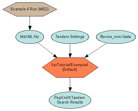
|
Example 4 Run
(MS2)
Summary View |
XarTutorial/Example4
(Default)
Summary View |
Referencing files for Data objects
The connection between the two runs is the Example4.mzXML
file. It is the output of the run described by Example4.xar.xml. It is the
input to a search run which has a xar.xml generated by the data pipeline, named
XarTutorial\xtandem\Default\Example4.search.xar.xml. The CPAS system knows
these two experiment runs are linked because the marked output of the first run
is identified as a starting input to the second run. The file Example4.mzXML
is represented in the xar object model as a Data object with a DataFileUrl
property containing the path to the file. Since both of the runs are referring
to the same physical file, there should be only one Data object created. The
${AutoFileLSID} substitution template serves this purpose. ${AutoFileLSID}
must be used in conjunction with a DataFileUrl value that gives a path to a
file relative to the xar.xml file’s directory. At load time the CPAS loader
checks to see if an existing Data object points to that same file. If one
exists, that object’s LSID is substituted for the template. If none exists,
the loader creates a new Data object with a unique LSID. Sharing the same LSID
between the two runs allows the CPAS system to show the linkage between the
two, as in Figure 4.
Table 4: Example 4 LCMS2 Experiment description
|
Example4.xar.xml
The OutputDataLSID of the step that produces the mzXML
file uses the ${AutoFileLSID}
template. A second parameter, OutputDataFileTemplate, gives the relative
path to the file from the xar.xml’s directory (in this case the file is in
the same directory).
|
<exp:Protocol rdf:about="${FolderLSIDBase}:ConvertToMzXML">
<exp:Name>Convert to
mzXML</exp:Name>
<exp:ApplicationType>ProtocolApplication</exp:ApplicationType>
<exp:MaxInputMaterialPerInstance>0</exp:MaxInputMaterialPerInstance>
<exp:MaxInputDataPerInstance>1</exp:MaxInputDataPerInstance>
<exp:OutputMaterialPerInstance>0</exp:OutputMaterialPerInstance>
<exp:OutputDataPerInstance>1</exp:OutputDataPerInstance>
<exp:OutputDataType>Data</exp:OutputDataType>
<exp:ParameterDeclarations>
<exp:SimpleVal
Name="ApplicationLSIDTemplate"
OntologyEntryURI="terms.fhcrc.org#XarTemplate.ApplicationLSID"
ValueType="String">${RunLSIDBase}:${InputLSID.objectid}.DoConvertToMzXML</exp:SimpleVal>
<exp:SimpleVal
Name="ApplicationNameTemplate" OntologyEntryURI="terms.fhcrc.org#XarTemplate.ApplicationName"
ValueType="String">Do conversion to MzXML</exp:SimpleVal>
<exp:SimpleVal
Name="OutputDataLSIDTemplate"
OntologyEntryURI="terms.fhcrc.org#XarTemplate.OutputDataLSID"
ValueType="String">${AutoFileLSID}</exp:SimpleVal>
<exp:SimpleVal
Name="OutputDataFileTemplate"
OntologyEntryURI="terms.fhcrc.org#XarTemplate.OutputDataFile"
ValueType="String">Example4.mzXML</exp:SimpleVal>
<exp:SimpleVal
Name="OutputDataNameTemplate"
OntologyEntryURI="terms.fhcrc.org#XarTemplate.OutputDataName"
ValueType="String">MzXML file</exp:SimpleVal>
</exp:ParameterDeclarations>
</exp:Protocol>
|
|
Example4.search.xar.xml
Two of the protocols in the generated xar.xml use the
${AutoFileLSID} template including the Convert to PepXml step shown. But
note here that the OutputDataFileTemplate
parameter is declared but does not have a default value.
|
<exp:Protocol
rdf:about="${FolderLSIDBase}:MS2.ConvertToPepXml">
<exp:Name>Convert To
PepXml</exp:Name>
<exp:ApplicationType>ProtocolApplication</exp:ApplicationType>
<exp:MaxInputMaterialPerInstance>0</exp:MaxInputMaterialPerInstance>
<exp:MaxInputDataPerInstance>1</exp:MaxInputDataPerInstance>
<exp:OutputMaterialPerInstance>0</exp:OutputMaterialPerInstance>
<exp:OutputDataPerInstance>1</exp:OutputDataPerInstance>
<exp:ParameterDeclarations>
<exp:SimpleVal
Name="ApplicationLSIDTemplate"
OntologyEntryURI="terms.fhcrc.org#XarTemplate.ApplicationLSID"
ValueType="String">${RunLSIDBase}::MS2.ConvertToPepXml</exp:SimpleVal>
<exp:SimpleVal
Name="ApplicationNameTemplate"
OntologyEntryURI="terms.fhcrc.org#XarTemplate.ApplicationName"
ValueType="String">PepXml/XTandem Search Results</exp:SimpleVal>
<exp:SimpleVal
Name="OutputDataLSIDTemplate"
OntologyEntryURI="terms.fhcrc.org#XarTemplate.OutputDataLSID"
ValueType="String">${AutoFileLSID}</exp:SimpleVal>
<exp:SimpleVal
Name="OutputDataFileTemplate"
OntologyEntryURI="terms.fhcrc.org#XarTemplate.OutputDataFile"
ValueType="String"/>
<exp:SimpleVal
Name="OutputDataNameTemplate"
OntologyEntryURI="terms.fhcrc.org#XarTemplate.OutputDataName"
ValueType="String">PepXml/XTandem Search
Results</exp:SimpleVal>
</exp:ParameterDeclarations>
<exp:Properties/>
</exp:Protocol>
|
|
The StartingInputDefintions use the ${AutoFileLSID}
template. This time the files referred to are in different directories from
the xar.xml file. The Xar load process turns these relative paths into
paths relative to the Pipeline root when checking to see if Data objects
already point to them.
|
<exp:StartingInputDefinitions>
<exp:Data rdf:about="${AutoFileLSID}">
<exp:Name>Example4.mzXML</exp:Name>
<exp:CpasType>Data</exp:CpasType>
<exp:DataFileUrl>../../Example4.mzXML</exp:DataFileUrl>
</exp:Data>
<exp:Data
rdf:about="${AutoFileLSID}">
<exp:Name>Tandem
Settings</exp:Name>
<exp:CpasType>Data</exp:CpasType>
<exp:DataFileUrl>tandem.xml</exp:DataFileUrl>
</exp:Data>
<exp:Data
rdf:about="${AutoFileLSID}">
<exp:Name>Bovine_mini.fasta</exp:Name>
<exp:CpasType>Data</exp:CpasType>
<exp:DataFileUrl>..\..\databases\Bovine_mini.fasta</exp:DataFileUrl>
</exp:Data>
</exp:StartingInputDefinitions>
|
|
The ExperimentLog section of this xar.xml uses the
optional CommonParametersApplied element
to give the values for the OutputDataFileTemplate parameters. This element
has the effect of applying the same parameter values to all
ProtocolApplications generated for the current action.
|
<exp:ExperimentLog>
<exp:ExperimentLogEntry
ActionSequenceRef="1"/>
<exp:ExperimentLogEntry
ActionSequenceRef="30">
<exp:CommonParametersApplied>
<exp:SimpleVal
Name="OutputDataFileTemplate"
OntologyEntryURI="terms.fhcrc.org#XarTemplate.OutputDataFile"
ValueType="String">Example4.xtan.xml</exp:SimpleVal>
</exp:CommonParametersApplied>
</exp:ExperimentLogEntry>
<exp:ExperimentLogEntry
ActionSequenceRef="40">
<exp:CommonParametersApplied>
<exp:SimpleVal
Name="OutputDataFileTemplate"
OntologyEntryURI="terms.fhcrc.org#XarTemplate.OutputDataFile"
ValueType="String">Example4.pep.xml</exp:SimpleVal>
</exp:CommonParametersApplied>
</exp:ExperimentLogEntry>
<exp:ExperimentLogEntry
ActionSequenceRef="50"/>
</exp:ExperimentLog>
|
After using the Data Pipeline to generate a pep.xml peptide
search result, some users may want to integrate the two separate connected runs
of Example 4 into a single run that starts with a sample and ends with the
peptide search results. Example 5 is the result of this combination. [Note:
Because of a bug in version 1.1 of CPAS, you must delete the
“XarTutorial/Example4 (Default)” run and then the “Example 4 Run (MS2)” run
before loading Example 5].
Combine
connected runs into an end-to-end run (Example 5)

|

|
Summary View |
Details View |
Table 5: Highlights of MS2 end-to-end experiment
description (Example5.xar.xml)
|
The protocols of example 5 are the union of the two sets
of protocols in Example4.xar.xml and Example4.search.xar.xml. A new run
protocol becomes the parent of all of the steps.
Note that the ActionDefinition section has one unusual
addition: the XTandemAnalyze step has both the MS2EndToEndProtocol (first)
step and the ConvertToMzXML steps as predecessors. This is because it takes
as inputs 3 files: the mzXML file output by step 30 and the tandem.xml and
bovine_mini.fasta files. The latter two files are not produced by any step
in the protocol and so must be included in the StartingInputs section.
Adding step 1 as a predecessor is the signal that the XTandemAnalyze step
uses StartingInputs.
|
<exp:ProtocolActionDefinitions>
<exp:ProtocolActionSet
ParentProtocolLSID="${FolderLSIDBase}:MS2EndToEndProtocol">
<exp:ProtocolAction
ChildProtocolLSID="${FolderLSIDBase}:MS2EndToEndProtocol"
ActionSequence="1">
<exp:PredecessorAction
ActionSequenceRef="1"/>
</exp:ProtocolAction>
<exp:ProtocolAction
ChildProtocolLSID="${FolderLSIDBase}:SamplePrep"
ActionSequence="10">
<exp:PredecessorAction
ActionSequenceRef="1"/>
</exp:ProtocolAction>
<exp:ProtocolAction
ChildProtocolLSID="${FolderLSIDBase}:LCMS2"
ActionSequence="20">
<exp:PredecessorAction
ActionSequenceRef="10"/>
</exp:ProtocolAction>
<exp:ProtocolAction
ChildProtocolLSID="${FolderLSIDBase}:ConvertToMzXML"
ActionSequence="30">
<exp:PredecessorAction
ActionSequenceRef="20"/>
</exp:ProtocolAction>
<exp:ProtocolAction
ChildProtocolLSID="${FolderLSIDBase}:XTandemAnalyze"
ActionSequence="60">
<exp:PredecessorAction
ActionSequenceRef="1"/>
<exp:PredecessorAction
ActionSequenceRef="30"/>
</exp:ProtocolAction>
<exp:ProtocolAction
ChildProtocolLSID="${FolderLSIDBase}:ConvertToPepXml"
ActionSequence="70">
<exp:PredecessorAction
ActionSequenceRef="60"/>
</exp:ProtocolAction>
<exp:ProtocolAction
ChildProtocolLSID="${FolderLSIDBase}:MarkRunOutput"
ActionSequence="1000">
<exp:PredecessorAction
ActionSequenceRef="70"/>
</exp:ProtocolAction>
</exp:ProtocolActionSet>
</exp:ProtocolActionDefinitions>
|
Describing pooling and fractionation
Some types of MS2 experiments involve combining two related
samples into one prior to running LCMS2. The original samples are dyed with
different markers so that they can be distinguished. Example 6 demonstrates
how to do this in a xar.xml.
Sample pooling
and fractionation (Example 6)

|
Details View |
Table 6: Describing pooling and fractionation
(Example6.xar.xml)
|
There are two different tagging protocols for the two
different dye types.
The PoolingTreatment protocol has a
MaxInputMaterialPerInstance of 2 and an Output of 1
|
<exp:Protocol
rdf:about="${FolderLSIDBase}:TaggingTreatment.Cy5">
<exp:Name>Label with Cy5</exp:Name>
<exp:ProtocolDescription>Tag
sample with Amersham CY5 dye</exp:ProtocolDescription>
…
</exp:Protocol>
<exp:Protocol rdf:about="${FolderLSIDBase}:TaggingTreatment.Cy3">
<exp:Name>Label with Cy3</exp:Name>
…
</exp:Protocol>
<exp:Protocol
rdf:about="${FolderLSIDBase}:PoolingTreatment">
<exp:Name>Combine tagged samples</exp:Name>
<exp:ProtocolDescription/>
<exp:ApplicationType/>
<exp:MaxInputMaterialPerInstance>2</exp:MaxInputMaterialPerInstance>
<exp:MaxInputDataPerInstance>0</exp:MaxInputDataPerInstance>
<exp:OutputMaterialPerInstance>1</exp:OutputMaterialPerInstance>
<exp:OutputDataPerInstance>0</exp:OutputDataPerInstance>
…
</exp:Protocol>
|
|
Both tagging steps are listed as having the start protocol
(action sequence =1) as predecessors, meaning that they take StartingInputs.
The pooling step lists both the tagging steps as
predecessors.
|
<exp:ProtocolActionDefinitions>
<exp:ProtocolActionSet
ParentProtocolLSID="${FolderLSIDBase}:Example_6_Protocol">
<exp:ProtocolAction
ChildProtocolLSID="${FolderLSIDBase}:Example_6_Protocol"
ActionSequence="1">
<exp:PredecessorAction
ActionSequenceRef="1"/>
</exp:ProtocolAction>
<exp:ProtocolAction
ChildProtocolLSID="${FolderLSIDBase}:TaggingTreatment.Cy5"
ActionSequence="10">
<exp:PredecessorAction
ActionSequenceRef="1"/>
</exp:ProtocolAction>
<exp:ProtocolAction ChildProtocolLSID="${FolderLSIDBase}:TaggingTreatment.Cy3"
ActionSequence="11">
<exp:PredecessorAction
ActionSequenceRef="1"/>
</exp:ProtocolAction>
<exp:ProtocolAction
ChildProtocolLSID="${FolderLSIDBase}:PoolingTreatment"
ActionSequence="15">
<exp:PredecessorAction
ActionSequenceRef="10"/>
<exp:PredecessorAction
ActionSequenceRef="11"/>
</exp:ProtocolAction>
|
|
The two starting inputs need to be assigned to specific
steps so that the xar records which dye was applied to which sample. So this
xar.xml uses the ApplicationInstanceCollection element of the
ExperimentLogEntry to specify which input a step takes. Since there is only
one instance of step 10 (or 20) there is one InstanceDetails block in the
collection. The InstanceInputs refer to an LSID in the
StartingInputDefinitions block. Instance-specific parameters could also be
specified in this section.
|
<exp:StartingInputDefinitions>
<exp:Material rdf:about="${FolderLSIDBase}:Case">
<exp:Name>Case</exp:Name>
</exp:Material>
<exp:Material rdf:about="${FolderLSIDBase}:Control">
<exp:Name>Control</exp:Name>
</exp:Material>
</exp:StartingInputDefinitions>
<exp:ExperimentLog>
<exp:ExperimentLogEntry
ActionSequenceRef="1"/>
<exp:ExperimentLogEntry
ActionSequenceRef="10">
<exp:ApplicationInstanceCollection>
<exp:InstanceDetails>
<exp:InstanceInputs>
<exp:MaterialLSID>${FolderLSIDBase}:Case</exp:MaterialLSID>
</exp:InstanceInputs>
</exp:InstanceDetails>
</exp:ApplicationInstanceCollection>
</exp:ExperimentLogEntry>
<exp:ExperimentLogEntry
ActionSequenceRef="11">
<exp:ApplicationInstanceCollection>
<exp:InstanceDetails>
<exp:InstanceInputs>
<exp:MaterialLSID>${FolderLSIDBase}:Control</exp:MaterialLSID>
</exp:InstanceInputs>
</exp:InstanceDetails>
</exp:ApplicationInstanceCollection>
</exp:ExperimentLogEntry>
<exp:ExperimentLogEntry
ActionSequenceRef="15"/>
|
Full Example: Lung Adenocarcinoma Study
description
The file LungAdenocarcinoma.xar.xml is a fully annotated
description of an actual study. It uses export format because it includes
custom properties attached to run outputs. Properties of generated outputs
cannot currently be described using log format.
Overview of Life Sciences IDs
The LabKey Server platform uses the emerging LSID standard (
http://www.omg.org/docs/dtc/04-05-01.pdf) for identifying entities in the database, such as experiment and protocol definitions. LSIDs are a specific form of URN (Universal Resource Name). Entities in the database will have an associated
LSID field that contains a unique name to identify the entity.
Constructing LSIDS
LSIDs are multi-part strings with the parts separated by colons. They are of the form:
urn:lsid:<AuthorityID>:<NamespaceID>:<ObjectID>:<RevisionID>
The variable portions of the LSID are set as follows:
- <AuthorityID>: An Internet domain name
- <NamespaceID>: A namespace identifier, unique within the authority
- <ObjectID>: An object identifier, unique within the namespace
- <RevisionID>: An optional version string
An example LSID might look like the following:
urn:lsid:genologics.com:Experiment.pub1:Project.77.3
LSIDs are a solution to a difficult problem: how to identify entities unambiguously across multiple systems. While LSIDs tend to be long strings, they are generally easier to use than other approaches to the identifier problem, such as large random numbers or Globally Unique IDs (GUIDs). LSIDs are easier to use because they are readable by humans, and because the LSID parts can be used to encode information about the object being identified.
Note: Since LSIDs are a form of URN, they should adhere to the character set restrictions for URNs (see http://www.zvon.org/tmRFC/RFC2141/Output/index.html). LabKey Server complies with these restrictions by URL encoding the parts of an LSID prior to storing it in the database. This means that most characters other than letters, numbers and the underscore character are converted to their hex code format. For example, a forward slash "/" becomes "%2F" in an LSID. For this reason it is best to avoid these characters in LSIDs.
The LabKey Server system both generates LSIDs and accepts LSID-identified data from other systems. When LSIDs are generated by other systems, LabKey Server makes no assumptions about the format of the LSID parts. External LSIDs are treated as an opaque identifier to store and retrieve information about a specific object. LabKey Server does, however, have specific uses for the sub-parts of LSIDs that are created on the LabKey Server system during experiment load.
Once issued, LSIDs are intended to be permanent. The LabKey Server system adheres to this rule by creating LSIDs only on insert of new object records. There is no function in LabKey Server for updating LSIDs once created. LabKey Server does, however, allow deletion of objects and their LSIDs.
AuthorityID
The Authority portion of an LSID is akin to the "issuer" of the LSID. In LabKey Server, the default authority for LSIDs created by the LabKey Server system is set via the Customize Site page on the Admin Console page. Normally this should be set to the host portion of the address by which users connect to the LabKey Server instance, such as proteomics.fhcrc.org.
Note: According to the LSID specification, an Authority is responsible for responding to metadata queries about an LSID. To do this, an Authority would implement an LSID resolution service, of which there are three variations. The LabKey Server system does not currently implement a resolution service, though the design of LabKey Server is intended to make it straightforward to build such a service in the future.
NamespaceID
The Namespace portion of an LSID specifies the context in which a particular ObjectID is unique. Its uses are specific to the authority. LSIDs generated by the LabKey Server system use this portion of the LSID to designate the base object type referred to by the LSID (for example, Material or Protocol.) LabKey LSIDs also usually append a second namespace term (a suffix) that is used to ensure uniqueness when the same object might be loaded multiple times on the same LabKey Server system. Protocol descriptions, for example, often have a folder scope LSID that includes a namespace suffix with a number that is unique to the folder in which the protocol is loaded.
ObjectID
The ObjectID part of an LSID is the portion that most closely corresponds to the "name" of the object. This portion of the LSID is entirely up to the user of the system. ObjectIDs often include usernames, dates, or file names so that it is easier for users to remember what the LSID refers to. All objects that have LSIDs also have a Name property that commonly translates into the ObjectID portion of the LSID. The Name property of an object serves as the label for the object on most LabKey Server pages. It's a good idea to replace special characters such as spaces and punctuation characters with underscores or periods in the ObjectID.
RevisionID
LabKey Server does not currently generate RevisionIDs in LSIDs, but can accept LSIDs that contain them.
LSID Example
Here is an example of a valid LabKey LSID:
urn:lsid:labkey.org:Protocol.Folder-2994:SamplePrep.Biotinylation
This LSID identifies a specific protocol for a procedure called biotinylation. This LSID was created on a system with the LSID authority set to labkey.org. The namespace portion indicates that Protocol is the base type of the object, and the suffix value of Folder-2994 is added so that the same protocol can be loaded in multiple folders without a key conflict (see the discussion on substitution templates below). The ObjectId portion of the LSID can be named in whatever way the creator of the protocol chooses. In this example, the two-part ObjectId is based on a sample preparation stage (SamplePrep), of which one specific step is biotinylation (Biotinylation).
LSID Substitution Templates
The extensive use of LSIDs in LabKey Server requires a system for generating
unique LSIDs for new objects. LSIDs must be unique because they are
used as keys to identify records in the database. These generated LSIDs
should not inadvertently clash for two different users working in
separate contexts such as different folders. On the other hand, if the
generated LSIDs are too complex – if, for example, they
guarantee uniqueness by incorporating large random numbers –
then they become difficult to remember and difficult to share among
users working on the same project.
LabKey Server allows authors of experiment description
files (
xar.xml
files) to specify LSIDs which include substitution
template values. Substitution templates are strings of the form
${<substitution_string>}
where
<substitution_string> is one of the
context-dependent values listed in the table below. When an experiment
description file is loaded into the LabKey Server database, the substitution
template values are resolved into final LSID values. The actual values
are dependent on the context in which the load occurs.
Unless otherwise noted, LSID substitution templates are supported in a
xar.xml file wherever LSIDs are used. This includes the following
places in a xar.xml file:
- The LSID value of the rdf.about
attribute. You can use a
substitution template for newly created objects or for references to
objects that may or may not exist in the database.
- References to LSIDs that already exist, such as
the ChildProtocolLSID
attribute.
- Templates for generating LSIDs when using the ExperimentLog
format (ApplicationLSID,
OuputMaterialLSID, OutputDataLSID).
A limited subset of the substitution templates are also supported in
generating object Name values when using the ExperimentLog format
(
ApplicationName,
OutputMaterialName,
and
OutputDataName).
These same templates are available for generating file names and file
directories (
OutputDataFile
and
OutputDataDir).
Collectively
these uses are listed as the Name/File ProtocolApplication
templates in the table below.
Note:
The following table lists the primitive, single component
substitution templates first. The most powerful and useful substitution
templates are compound substitutions of the simple templates. These
templates are listed at the bottom of the table.
Table: LSID
Substition Templates in LabKey Server
|
${LSIDAuthority}
|
|
|
Expands to
|
Server-wide value set on the Customize Site
page
under Site Administration. The default value is localhost.
|
|
|
Where valid
|
|
|
|
|
${LSIDNamespace.prefix}
|
|
|
Expands to
|
Base object name of object being identified by the LSID;
e.g.,
Material, Data, Protocol, ProtocolApplication,
Experiment, or ExperimentRun
|
|
|
Where valid
|
|
|
|
|
${Container.RowId}
${Container.path}
|
|
|
Expands to
|
Unique integer or path of project or folder into which
the
xar.xml is loaded. Path starts at the project and uses periods to
separate
folders in the hierarchy.
|
|
|
Where valid
|
- Any LSID
- Name/File ProtocolApplication templates
|
|
|
|
${XarFileId}
|
|
|
Expands to
|
Xar- + unique integer for xar.xml
file being loaded
|
|
|
Where valid
|
- Any LSID
- Name/File ProtocolApplication templates
|
|
|
|
${UserEmail},${UserName}
|
|
|
Expands to
|
Identifiers for the logged-on user initiating the
xar.xml
load
|
|
|
Where valid
|
- Any LSID
- Name/File ProtocolApplication templates
|
|
|
|
${ExperimentLSID}
|
|
|
Expands to
|
rdf:about value of the Experiment
node at the top
of the xar.xml being loaded
|
|
|
Where valid
|
- Any other LSID in the same xar.xml
- Name/File ProtocolApplication templates
|
|
|
|
${ExperimentRun.RowId}
${ExperimentRun.LSID}
${ExperimentRun.Name}
|
|
|
Expands to
|
The unque integer, LSID, and Name of the ExperimentRun
being loaded
|
|
|
Where valid
|
- LSID/Name/File ProtocolApplication templates that
are
part of that specific ExperimentRun
|
|
|
|
${InputName},${InputLSID}
|
|
|
Expands to
|
The name and lsid of the Material or Data object that is
the input to a ProtocolApplication being generated using ExperimentLog
format.
Undefined if there is not exactly one Material or Data
object that is
input.
|
|
|
Where valid
|
- LSID/Name/File ProtocolApplication templates that
have exactly one input, e.g., MaxInputMaterialPerInstance +
MaxInputDataPerInstance = 1
|
|
|
|
${InputLSID.authority}
${InputLSID.namespace}
${InputLSID.namespacePrefix}
${InputLSID.namespaceSuffix}
${InputLSID.objectid}
${InputLSID.version}
|
|
|
Expands to
|
The individual parts of an InputLSID, as defined above.
The
namespacePrefix is defined as the namespace
portion up to but not
including the first period, if any. The namepsaceSuffix
is the
remaining portion of the namespace after the first period.
|
|
|
Where valid
|
- LSID/Name/File ProtocolApplication templates that
have exactly one input, i.e., MaxInputMaterialPerInstance +
MaxInputDataPerInstance = 1
|
|
|
|
${InputInstance},${OutputInstance}
|
|
|
Expands to
|
The 0-based integer number of the ProtocolApplication
instance within an ActionSequence. Useful for any ProtocolApplication
template that includes a fractionation step. Note that InputInstance
is > 0 whenever the same Protocol is applied multiple times in
parallel. OutputInstance
is only > 0 in a fractionation step in which multiple outputs
are
generated for a single input.
|
|
|
Where valid
|
- LSID/Name/File ProtocolApplication templates that
are
part of that specific ExperimentRun
|
|
|
|
${FolderLSIDBase}
|
|
|
Expands to
|
urn:lsid:${LSIDAuthority}:
${LSIDNamespace.Prefix}.Folder-${Container.RowId}
|
|
|
Where valid
|
|
|
|
|
|
|
${RunLSIDBase}
|
|
|
Expands to
|
urn:lsid:${LSIDAuthority}:${LSIDNamespace.Prefix}
.Run-${ExperimentRun.RowId}
|
|
|
Where valid
|
|
|
|
|
${AutoFileLSID}
|
|
|
Expands to
|
urn:lsid:${LSIDAuthority}
:Data.Folder-${Container.RowId}-${XarFileId}:
See Data object in next section for behavior
and usage
|
|
|
Where valid
|
|
Common Usage
Patterns
In general, the primary object types in a Xar file use the following
LSID patterns:
Experiment, ExperimentRun, Protocol
These three object types typically use folder-scoped LSIDs that look
like
${FolderLSIDBase}:Name_without_spaces
In these LSIDs the object name and the LSID’s objectId are
the same except for the omission of characters (like spaces) that would
get encoded in the LSID.
ProtocolApplication
A ProtocolApplication is always part of one and only one ExperimentRun,
and is loaded or deleted with the run. For ProtocolApplications, a
run-scoped LSID is most appropriate, because it allows multiple runs
using the same protocol to be loaded into a single folder. A run-scoped
LSID uses a pattern like
${RunLSIDBase}:Name_without_spaces
Material
Material objects can be divided into two types: starting Materials and
Materials that are created by a ProtocolApplication. If the Material is
a starting material and is not the output of any ProtocolApplication,
its scope is outside of any run. This type of Material would
normally have a folder-scoped LSID using ${FolderLSIDBase}. On the
other hand, if the Material is an output of a ProtocolApplication, it
is scoped to the run and would get deleted with the run. In this case
using a run-scoped LSID with ${RunLSIDBase} would be more appropriate.
Data
Like Material objects, Data objects can exist before any run is
created, or they can be products of a run. Data objects are also
commonly associated with physical files that are on the same file share
as the xar.xml being loaded. For these data objects associated with
real existing files, it is important that multiple references to the
same file all use the same LSID. For this purpose, LabKey Server provides the
${AutoFileLSID} substitution template, which works somewhat differently
from the other substitution templates. An ${AutoFileLSID} always has an
associated file name on the same object in the xar.xml file:
- If the ${AutoFileLSID} is on a starting Data object, that
object also has a DataFileUrl element.
- If the ${AutoFileLSID} is part of a
XarTemplate.OutputDataLSID parameter, the XarTemplate.OutputDataFile
and XarTemplate.OutputDataDir specify the file
- If the ${AutoFileLSID} is part of a DataLSID (reference),
the DataFileUrl attribute specifies the file.
When the xar.xml loader finds an ${AutoFileLSID}, it first calculates
the full path to the specified file. It then looks in the database to
see if there are any Data objects in the same folder that already point
to that file. If an existing object is found, that object’s
LSID is used in the xar.xml load. If no existing object is found, a new
LSID is created.
Run Groups
Run groups allow you to assign various types of runs (MS1, MS2, Luminex, etc) to different groups. You can define any groups that you like. Some examples might be separate groups for case and control, a group to hold all of your QC runs, or separate groups for each of the different instruments you use in the lab. Run groups are scoped to a particular folder inside of LabKey Server.
Create Run Groups and Associate Runs with Run Groups
From a list of runs, select the runs you want to add to the group and click on the "Add to run group" button. You'll see a popup menu. If you haven't already created the run group, click on "Create new run group."

This will bring you a page that asks you information about the run group. You must give it a name, and can provide additional information if you like. Clicking on "Submit" will create the run group, add the runs you selected to it. It will then return you to the list of runs.
Continue this process to define all the groups that you want. You can also add runs to existing run groups.
The "Run Groups" column will show all of the groups to which a run belongs.
Viewing Run Groups
You can click on the name of a run group in the "Run Groups" column within a run list to see its details. You can also add the "Run Group" web part to your folder, or access it through the Experiment tab.
You can edit the run group's information, as well as view all of the run group's runs. LabKey Server will attempt to determine the most specific type of run that describes all of the runs in the list and give you the related set of options.
Viewing Group Information from an Individual Run
From either the text or graphical view of an experiment run, you have access to a list of all the run groups in the current folder. By default, the Run Groups list is collapsed, but you can click to expand. You can toggle the run's group membership by checking or unchecking the checkboxes.

Filtering a Run List by Run Group Membership
You can add columns to your list of runs that let you filter by run group membership. Click on "Customize View". Expand the "Run Groups" node in the tree. Select the group or groups that you want to add to your list and click on "Add". Click on the "Save" button.
Your run list will now include columns with checkboxes that show if a run belongs to the group. You can toggle the checkboxes to change the group memberships. You can also add a filter where the value is equal to TRUE or FALSE to restrict the list of runs based on group membership.

Portal
The Portal Module provides a Portal page that can be customized with Web Parts. Without Portal services, you cannot add Web parts. The home page for all four
LabKey Applications is the Portal page.
You can create a Custom Folder that does not include the Portal Module and thus does not have a Portal Page. If you do so, the UI for each Module's services will be available only on the tab corresponding to each included module. Web Parts will not be available from the Add Web Parts drop-down menu because this menu is only available on a Portal page.
Sub-Inventories
Application Inventory
Modules form the functional units of LabKey Systems. Modules provide task-focused features for storing, processing, sharing and displaying files and data.
Applications aggregate the features of multiple Modules into comprehensive suites of tools. Existing Application suites can be enhanced through customization and the addition of extra Modules.
Web Parts provide UI access to Module features. They appear as sections on a Folder's Portal Page and can be added or removed by administrators.
LabKey Application Inventory
Collaboration: The Collaboration Application helps you build a web site for publishing and exchanging information. Depending on how your project is secured, you can share information within your own group, across groups, or with the public. Included Modules:
Flow Cytometry: The Flow Application manages compensated, gated flow cytometry data and generates dot plots of cell scatters. Included Modules:
MS1 The MS1 Application allows you to combine MS1 quantitation results with MS2 data.
MS2: The MS2 Application (also called CPAS or the MS2 Viewer) provides MS2 data mining for individual runs across multiple experiments. It supports multiple search engines, including X!Tandem, Sequest, and Mascot. The MS2 Application integrates with existing analytic tools like PeptideProphet and ProteinProphet. Included Modules:
Microarray: The Microarray application allows you to process and manage data from microarray experiments.
Study: The Study Application manages parameters for human studies involving distributed sites, multiple visits, standardized assays, and participant data collection. The Study Application provides specimen tracking for samples collected at site visits. Included Modules:
Module Inventory
LabKey Module Inventory
Note on Accessing Modules and Their Features: All modules are installed by default with your Server. However, each module and its tools are only available in a particular Folder when your Admin sets them up. Ask your Admin which modules and tools are set up in your Folder.
This inventory lists all Modules and the Web Parts they provide. Wide (left side) Web Parts are listed first. Narrow (right side) web parts are listed second and are indicated by the marker "-> Narrow."
BioTrue The BioTrue Module allows periodically walking a BioTrue CDMS, and copying the files down to a file system.
- BioTrue Connector Overview (Server Management/ BioTrue Connector Dashboard)
Demo The Demo Module helps you get started building your own LabKey Server module. It demonstrates all the basic concepts you need to understand to extend LabKey Server with your own module.
- Demo Summary
- Demo Summary ->Narrow
Experiment: The Experiment module provides annotation of experiments based on FuGE-OM standards. This module defines the XAR (eXperimental ARchive) file format for importing and exporting experiment data and annotations, and allows user-defined custom annotations for specialized protocols and data.
- Experiment Runs
- Experiments
- Lists
- Sample Sets
- Single List
- Experiments -> Narrow
- Protocols -> Narrow
- Sample Sets -> Narrow
File Upload and Sharing: The FileContent Module lets you share files on your LabKey Server via the web. It lets you serve pages from a web folder.
Flow Cytometry: The Flow Module supplies Flow-specific services to the Flow Application.
- Flow Analysis (Flow Analysis Folders)
- Flow Analysis Scripts
- Flow Overview (Experiment Management)
Issues: The Issues module provides a ready-to-use workflow system for tracking tasks and problems across a group.
Messages: The Messages module is a ready-to-use message board where users can post announcements and files and participate in threaded discussions.
MS1 The MS1 Module supplies MS1-specific services to the MS1 Application.
Proteomics The MS2 Module supplies MS2-specific services to the MS2/CPAS Application.
- MS2 Runs
- MS2 Runs, Enhanced
- MS2 Sample Preparation Runs
- Protein Search
- MS2 Statistics ->Narrow
- Protein Search ->Narrow
NAb The NAB module provides tools for planning, analyzing and organizing experiments that address Neutralizing Antibodies. No Web Parts provided. Access NAB services via a custom Tab in a Custom Folder.
Portal. The Portal Module provides a Portal page that can be customized with Web Parts.
Pipeline: The Data Pipeline module uploads experiment data files to LabKey. You can track the progress of uploads and view log and output files. These provide further details on the progress of data files through the pipeline, from file conversion to the final location of the analyzed runs.
Query The query module allows you to
create customized Views by
filtering and sorting data. Web Part provided:
Study The Study Module supplies Study-specific services to the Study Application.
- Assay Details
- Assay List
- Datasets
- Enrollment Report
- Reports and Views
- Specimens
- Study Design (Vaccine Study Protocols)
- Study Overview
- Study Protocol Summary
- Vaccine Study Protocols
- Reports and Views -> Narrow
- Specimens -> Narrow
Wiki: The Wiki module provides a simple publishing tool for creating and editing web pages on the LabKey site. The Wiki module includes the Wiki, Narrow Wiki, and Wiki TOC web parts.
- Wiki
- Wiki -> Narrow
- Wiki TOC -> Narrow
Web Part Inventory (Basic Wiki Version)
LabKey Web Part Inventory
The following tables list available Web Parts and the Module that supplies each Web Part.
Wide Web parts are listed first. When included on a page, these typically display on the leftmost 2/3rds of the page. Narrow web parts are listed second and display on the rightmost 1/3rd of the page.
Wide Web Parts
Narrow Web Parts
Web Part Inventory (Expanded Wiki Version)
LabKey Web Part Inventory
The following tables list available Web Parts and the Module that supplies each Web Part.
Wide Web parts are listed first. When included on a page, these typically display on the leftmost 2/3rds of the page. Narrow web parts are listed second and display on the rightmost 1/3rd of the page.
In some cases, the web part name displayed in the UI does not match the web part name selected by Administrators during the process of adding web parts. In such cases, the displayed name is listed in single quotes after the name selected by Administrators from the "Add Web Part" drop-down menu.
Wide Web Parts
| | | |
|---|
| Web Part Name | Source Module | Brief Description |
| Assay Details | Study | |
| Assay List | Study | List of available assays with data that can be uploaded (HUH?) |
| BioTrue Connector Overview | BioTrue | Reads files from a Biotrue CDMS server |
| Contacts | Portal | List of users on this server. Not yet in Portal |
| Data Pipeline | Pipeline | |
| Datasets | Study | Datasets included in this Study |
| Demo Summary | Demo | |
| Enrollment Report | Study | Simple graph of enrollment over time |
| Experiment Runs | Experiment | |
| Experiments | Experiment | List of experiments. Not very used. |
| Files | File Upload and Sharing | Lists a set. (what is a set?) |
| Flow Analysis 'Flow Analysis Folders' | Flow Cytometry | Appears in the UI as: "Flow Analysis Folders" |
| Flow Analysis Scripts | Flow Cytometry | |
| Flow Overview 'Experiment Management' | Flow Cytometry | Appears in the UI as: "Experiment Management" |
| Issues | Issues | Summary of Issues in the current folder's Issue Tracker. |
| Lists | Experiment | List of custom Lists in this folder |
| MS2 Runs | Proteomics | |
| MS2 Runs (Enhanced) | Proteomics | List of MS2 runs. |
| MS2 Sample Preparation Runs | Proteomics | List of sample prep runs. Not sure usage of this (ask josh) |
| Messages | Messages | Messages (aka Announcements) are found in this folder. |
| Messages List | Messages | Same as above, but without any message details. |
| Protein Search | Proteomics | |
| Query 'Queries' | Query | Shows results of a query as a grid. Appears in the UI as "Queries" |
| Reports 'Reports and Views' | Study | List of Reports and Views for this study. Appears in the UI as: "Reports and Views" |
| Sample Sets | Experiment | Sets of samples that have been uploaded for inclusion in assays/experiments |
| Search | Portal | Text box to search wiki & other modules for a search string |
| Specimens (Wide) | Study | List of specimens by type |
| Study Designs 'Vaccine Study Protocols' | Study | List of protocols that have been defined. These may or may not have been turned into real studies. Appears in the UI as: Vaccine Study Protocols |
| Study Overview | Study | Management links for a study folder. |
| Study Protocol Summary | Study | Overview of a Study Protocol (number of participants, etc). |
| Wiki | Wiki | |
Narrow Web Parts
| | | |
|---|
| Web Part Name | Source Module | Brief Description |
| Experiments | Experiment | List of experiments. Not very used. |
| Files | File Upload and Sharing | Lists a set. (what is a set?) |
| MS2 Statistics | Proteomics | Statistics on how many runs have been done on this server, etc. |
| Narrow Demo Summary 'Demo Web Part' | Demo | Appears in the UI as "Demo Web Part." |
| Narrow Search | Portal | Text box to search wiki & other modules for a search string |
| Narrow Wiki | Wiki | |
| Protein Search | Proteomics | Form for finding protein information. |
| Protocols | Experiment | |
| Reports | Study | List of Reports and Views for this study. Appears in the UI as "Reports and Views" |
| Sample Sets | Experiment | Sets of samples that have been uploaded for inclusion in assays/experiments |
| Specimens | Study | List of specimens by type |
| Wiki TOC | Wiki | Table of Contents for wiki pages. |
Collaboration
Overview
[Community Forum] [Demo]
LabKey Server provides a robust infrastructure for web-based collaboration. Building blocks include "anywhere" database access, file sharing, easy-to-manage security groups, authentication, auditing, message boards, issue trackers and wikis.
LabKey Server allows integration of many different types of data on one platform -- from descriptive study observations to large quantities of assay data. But data integration is only part of the story. Modern research teams need to work with their integrated datasets collaboratively, no matter the number or location of team members. LabKey Server helps such teams collaborate by providing web-based sharing, editing and display of both data and files.
Your team can build a data portal on top of LabKey Server to allow your users to see, share and/or update live data and visualizations of this data. Labkey's built-in wiki tool allow you to custom-tailor the way your portal displays and organizes information for your data-sharing community -- however large, dispersed or specialized that community may be. Depending on how you secure your project, you can share information within your own group, across groups, or with the public. You can add issue trackers to track project tasks or or message boards to facilitate discussions of research data among colleagues.
Documentation Topics
Create a Collaboration Folder
Step 1: Create or Customize
You can gain access to collaboration services in several ways.
- Create a new project or folder and set the folder type to "Collaboration". Your new project or folder will include a Portal page, wiki, issue tracker, message board, file-sharing and search capabilities.
- Customize the type of an existing folder. Select the project or folder in the left navigation pane and choose "Manage Project->Customize Folder". Set the folder type option to "Collaboration". Alternatively, you can also select the "Custom" type if you would like to display tabs for each module or have full access to all modules' web parts.
Step 2: Add Web Parts
Once your folder has access to collaboration services, you typically need to add tools to expose these services in the folder's UI.
Admins Add Web Parts to the Portal page to supply tools for using collaboration services. In the drop-down menu that appears at the bottom of the Portal page's content, select the web part that you want to add and click Add Web Part. When you add a web part, you are adding a component that allows you and your users to view and interact with the data in your project or folder.
Issues
The LabKey Issues module provides an issue tracker, a centralized workflow system for tracking issues or tasks across the lifespan of a project. Users can use the issue tracker to assign tasks to themselves or others, and follow the task through the work process from start to completion.
Note: Issue trackers on your LabKey Server installation are stored in the same database, and issue numbers are assigned sequentially as issues are added, regardless of the project or folder to which they belong. So issue numbers in your list may not be in sequence, if issues have been added to issue trackers in other projects in the interim.
Topics
Using the Issue Tracker
Issue Workflow
An issue has one of three possible states: it may be open, resolved, or closed.
Opening, Updating, and Assigning Issues
When you open or update an issue, you can assign it to another user (or to yourself). The Assigned To list includes all users who are members of groups defined in the project containing the Issues module. It also includes all site administrators. If an issue is opened by a user who is not a member of a group in that project, that user also appears in the Assigned To list.
If you want to include a particular user in the Assigned To list, you should add that user to a group that's defined on the project. For example, you can add the user to the default Users group that's defined for every new project.
Make sure that the group to which you add a user has at least write permissions (i.e., role is set to Editor) for the project or folder containing the Issues module. Otherwise you will be able to assign issues to that user, but they will not be able to update the issue.
After you assign an issue to a user, the system will send an email notification to that user, and the issue will appear in that user's list of issues.
If you want to reassign an issue, modify a field, or add further information to the description body, you can update the issue. You can update an open or a resolved issue. Updating an issue does not change its status.
Resolving an Issue
When an issue is assigned to you, you can assign it to someone else or resolve it in some manner. Options for resolution include: Fixed, Won't Fix, By Design, Duplicate, or Not Repro (meaning that the problem can't be reproduced by the person investigating it).
When an issue is resolved, its status is marked as resolved, and the issue tracker automatically assigns it back to the person who opened it (although you can choose to override this default assignment). This person can choose to either close the issue, if they are satisfied with the resolution, or re-open the issue, if they are not satisfied with the resolution.
Closing an Issue
When a resolved issue is assigned back to you, you can verify that the resolution is satisfactory, then close the issue. Closed issues remain in the Issues module, but they are no longer assigned to any individual, so they do not appear in lists that show open or resolved issues by user.
The Issues Grid
The Issues grid displays a list of the issues in the issue tracker. From the grid, you can sort and filter the list (see Selecting, Sorting & Filtering for more information on working with grid views).
Note: If there are more than 1000 issues, only the first 1000 are displayed in the grid. To display issues not included in this set, click the Show All Records button. You can also use the filtering and sorting buttons on the grid to display a different subset.
From the Issues grid, you can also:
- Export:
- All issues to Excel
- All issues to a text file
- As Web Query
- Print the current list of issues
- View the details for two or more issues on a single page
- Specify your email preferences for issues
- Create custom views
- Create an R view
Exporting to an Excel File, Text File or Web QueryClick the Export button and:
- Choose the Export All to Excel drop-down menu to export all of the issues in the issue tracker to an Excel file that you can view or save.
- Choose the Export All to Text drop-down menu to export all issues to a tab-separated values (.tsv) file.
- Choose the Export Web Query (.iqy) drop-down menu to export all issues as a web query.
View Selected DetailsTo view the details pages for two or more issues, select the desired issues in the grid and click View Selected Details. This function is useful for comparing two or more related or duplicate issues on the same screen.
Specify Email Preferences
Click the Email Preferences button to specify how you prefer to receive workflow email from the issue tracker. You can elect to receive no email, or you can select one or more of the following options:
- Send me email when an issue is opened and assigned to me
- Send me email when an issue that's assigned to me is modified
- Send me email when an issue I opened is modified
- Send me email notifications when I enter/edit an issue
Create Custom ViewsYou can use the LabKey Query module to create custom views on the issue tracker. See Custom Grid Views for more information on creating custom views.
Create R Views
If you have R configured on your LabKey Server, you can create an R view on the issue tracker. Select the Views button and choose Create R View from the drop-down menu. Saved R Views also appear under the Views drop-down menu (e.g., "Issues by Area").
Administering the Issue Tracker
A user with admin privileges can customize the issue tracker in the following ways:
- By defining the selection values that appear in the drop-down lists when an issue is being edited
- By specifying which fields must be completed in order for a user to submit an issue
- By defining custom columns
To customize the issue tracker, click the
Admin button on the issues list page.
Defining Selection Values
You can define selection values for the following built-in drop-down fields:
- Types: the type of issue or task.
- Areas: the area or category under which this issue falls
- Priorities: the importance of this issue
- Milestones: the targeted deadline for resolving this issue
- Resolutions: ways in which an issue may be resolved
You can also add custom fields in the
Custom Columns section of the admin page, and then specify selection values for those columns.
You can specify a default selection value for any field by clicking the [set] link next to that value. A new issue will display the default value for that field. To remove the default value, click the [clear]
button. The current default value is shown in boldface, as shown for the Resolutions field in the following image.

Specifying Required Fields
You can specify that a field must have a value before a new issue can be submitted. By default the Title and Assigned To fields are required; the admin page also gives you the option to require the Type, Area, Priority, Milestone, and Notify List fields, as well as any custom columns you add.
When a user creates or edits an issue, required fields are marked with a red asterisk (*).
Defining Custom Columns
You can add custom fields to the issue tracker on the Admin page. These fields will be displayed for viewing or editing when an issue is opened, updated, resolved, or closed.
There are two integer and two string custom fields available to you. If you check the Use pick list for this column field, you can add selection values for the custom field as described above. You can also specify whether the custom field is a required field.
Issues Web Part
The Issues web part displays a summary of the issues by user on a Portal page. A user may click the [view open issues] link to navigate to the full list of issues. Note that a given project or folder has only one associated Issues module, so if you add more than one Issues web part to a Portal page, both will display the same data.
Messages
The Messages module provides a message board.
A workgroup or user community can use the LabKey message board to post announcements and files and to carry on threaded discussions. The message board is useful for discussing ongoing work, answering questions and providing support, and posting documents for project users.
Topics covered in this section
Topics covered elsewhere
Using the Message Board
As a user of a message board, you can post new messages, edit existing messages (depending on your security privileges), and configure your preferences for receiving email from the message board.
For information on administering the message board, see Administering the Message Board.
Posting New Messages
You can post a new message to a message board if you have Author permissions or higher on the project or folder. When a logged-in user posts a message, their user name or email address will be displayed next to the message title. If the anonymous user (as a member of the Guests or Anonymous group) has sufficient privileges to post a message, no name appears next to the message title.
When you post a new message, you can optionally add a date to the Expires field. Once the expiration date has passed, the message will no longer appear in the web part on the portal page, but it will still appear in the full message list. You can use this feature to display only the most relevant or urgent messages on the Portal page, while still preserving all messages. If you leave the Expires field blank, the message will never expire.
To enter a date for the Expires field, format the date as mm/dd/yy or mm/dd/yyyy.
Enter the content of your message in the Body field. You can specify whether the message should be rendered as plain text with links, as wiki syntax, or as HTML.
To add an attachment, click the Browse button to locate the file you want to attach. Attachments should not exceed 250MB per message.
Editing Messages
To edit a message, click the [View Thread] link, then click [Edit Message] to edit the original message, or [Edit Response] to edit a message response.
To edit a message that you have posted, you must have at least Author permissions. To edit a message that someone else has posted, you must have at least Editor permissions.
When you edit a message, you can set, modify, or remove the expiration date.
Responding to Messages
To post a response to a message, click the [View Thread] link, then click the Post a Response button. Responses are stored with the original message as a single thread, so all discussion about a topic stays together.
You can respond to a message if you have at least Author permissions on the project or folder.
Responses are not displayed by the web part or in the full message list in the module; you must view the message thread to see any responses to it.
Configuring Email Preferences
You can sign up to receive email notifications when new messages or responses are posted to a message board.
The message board administrator can specify default email preferences for the project. Each user can choose to override the administrator's setting.
To set your email preferences, click the [Email Preferences] link at the top right of the Messages web part. You can elect to receive email notifications for all posts, for responses to threads you've posted to only, or not at all (the default option).
You can also elect to receive an email each time a message is posted, or a single digest mail that summarizes all posts for that day.
Maximizing the Message Board
If you are on a Portal page, you can quickly navigate to a full-page Message Board by clicking on the square box on the top right corner of the Messages Web Part. This box represents the "maximize" button.
Administering the Message Board
A project administrator can customize a message board to meet the needs of the workgroup. The administrator can also set email preferences for message board users.
Message Board Web Parts
A project administrator can add message board web parts to the Portal page. The message board web parts include the Messages and Messages List parts:
- The Messages web part displays the full text of current messages on the Portal page. Each message is labeled with its author and the date it was posted, and includes a link to view or respond to the message.
- The Messages List displays a grid view of all messages posted on this message board. The grid can be sorted and filtered.
Customizing the Message Board
To customize the message board, click the "customize" link. The available settings are as follows:
Board name: The name for this message board, which appears at the top of the page.
Conversation name: The term used by the message board to refer to a conversation (for example, you might change this setting to thread).
Conversation sorting: Specifies how conversations are sorted on the home page of the Messages module or in one of the Messages web parts. The Initial Post setting sorts with the oldest message at the top. The Most Recent Post setting sorts with the newest message at the top.
Security: Specifies whether special security is in place for the message board, beyond the permissions on the folder. By default, message board security is set to Off. If message board security is turned on, a conversation is visible only to users with editor permissions or above and to users who have been explicitly added to the members list for a conversation (see below for more information about the members list). Messages posted to a secure message board cannot be edited after posting, and message content is never sent over email, even if users have set their email preferences to receive email.
Allow Editing Title: Specifies whether the title of a message can be edited after the message is posted. Note that this only applies to message boards where the Security setting is set to Off; if the message board is secured, the [edit] link does not appear.
Include Member List: Specifies whether the member list field appears when a message is being created or edited. The member list is a list of email addresses of users to receive email notification when the message is posted.
The member list behaves somewhat differently depending on whether message board security is off or on. If the message board is not secured, you can add to the member list any site user who has permissions to read the message board. In this way you can send an email notification to a user without specifying an email preference for them.
If the message board is secured, a message is private to users with editor permissions or above, and to users listed on the members list. That is, you can use the members list to make a message visible to a user who does not have editor permissions on the message board.
Include Status: Displays a drop-down list in insert or edit mode that indicates the status of a message, for workflow applications. Status options are Active and Closed.
Include Expires: Displays a date field in insert or edit mode that indicates when a message expires. After a message expires, it is no longer displayed on the Messages home page or in the Messages web part. However, it still appears in the messages list.
Include Assigned To: Displays a drop-down list of project members to whom the message can be assigned, as a task or workflow item. You can specify a default value for all new messages.
Include Format Picker Displays a drop-down list of options for message format: Wiki Page, HTML, or Plain Text. If the format picker is not displayed, new messages are posted as plain text.
Administering Email Preferences
Users who have read permissions on a message board can choose to receive emails containing the content of messages posted to the message board. A user can choose to receive email notifications for all conversations, only for conversations they've posted to, or not at all. Additionally, they can specify how they should receive emailed content: with an email for each posted message, or as a compiled digest of the day's messages. The user sets their preferences on the Email Preferences page (see Using the Message Board).
As project administrator, you can set default email preferences for emailing project users who have access to the message board. You can also change email preferences for individual users. Any user can override the preferences you set for them if they choose to do so.
To manage users' email preferences, click the "email admin" link.
Folder Default Settings
At the top of the Admin Email Preferences page, you'll see a drop-down list where you can specify the default email preferences for project members for this message board. The option that you select as the default preference determines how members will receive email if they do not specify their own email preferences.
Specifying default email preferences is useful if, for example, you are using the message board to disseminate information to the workgroup. Project members who forget to set their own email preferences or don't know how can still stay up-to-date on conversations.
The possible settings for the default email preference are:
- No email: Emails are never sent when messages are posted.
- All conversations: An email is sent for each message posted to the message board.
- My conversations: An email is sent only if the user has posted a message to the conversation.
- Daily digest of all conversations: A digest email is sent for all conversations.
- Daily digest of my conversations: A digest email is sent only for conversations to which the user has posted messages.
The default setting for the default preference is
My conversations. In other words, if you don't change this setting for the message board, by default project members will receive email notifications for any conversation to which they post a message.
Any member can override the message board default setting and choose to receive more or fewer email notifications. The first time a project member manages their own email preferences for the message board, they will see their preferences set to the default email preference.
Note: The default email preference setting applies only to project members. Other users who have access to the message board can define their own email preferences; their email delivery will not be affected by changing the default email preference.
Email Preferences Table
The Admin Email Preferences page displays a table of message board users and their email preferences. These users may fall into one of two categories:
- Project members: Project members are users who belong to a security group defined on the project. All project members appear in the email preferences table, for every message board in the project.
- Other users: Site users who have not been explicitly added to a project group, but who have an interest in a particular message board and have set their preferences to receive email.
The table displays these fields:
- Identifying fields: Email, FirstName, LastName, and DisplayName.
- Email Option: This field shows the current email preference for each user. If the user is a project member and has not specified an email preference, the email option appears as <project default>, indicating that this user will receive email according to the option set for the default email preference.
- Last Modified By: This field shows the last person to modify the email preference for this user. You can use this field to determine whether the user has specified an email preference, in which case you most likely do not want to override it.
- Project Member: This field indicates whether this user is a member of the project. If the value for this field is No, it means that this user is not a project member but has specified an email preference for the message board.
Bulk EditClick the Bulk Edit button to change user email preferences individually. Use caution in changing preferences; in most cases you will not want to override the user's preference, if the user has specified one.
Message Board Security
Note: Consider security settings for your message board carefully. A user with Editor permissions can edit any message posted to the message board. A user with Author permissions can edit their own messages, unless that user is anonymous. You may want to restrict anonymous users from posting to the message board at all by setting permissions for the Guests (Anonymous) group to Reader or No Permissions. For more information on setting permissions, see Configuring Permissions.
Contacts
NB: Today, the Contacts Web Part is only available when you create a Custom-Type Folder or Project. In the future it will become part of the Portal Module. At that point, the Web Part will be available any time the Portal Module is available.
The Contacts web part displays contact information for users who are members of the project's Users group. Only members of the Users group are displayed in this web part. A new project contains a Users group by default, but if the group has been deleted, or if you are working in the Home project, you'll need to create a group named Users and add to it the users whose contact info you want to display.
The Contacts web part displays the contact information that each user has entered for themselves in their account details. To access your account details, make sure you are logged in to the LabKey Server installation, then click My Account at the top right corner of any page to show your contact information. You can edit your contact information from this page, except for your email address. Because your email address is your LabKey user name, you can't modify it here. To change your email address, see your administrator.
Wiki
A wiki is a hierarchical collection of documents that multiple users can edit. Wiki pages can be written in HTML, plain text or a specialized wiki language. On LabKey Server, you can use a wiki to include formatted content in a project or folder. You can even embed live data in this content.
Wiki Admin Guide
This Wiki Admin Guide will help you set up a wiki using web parts. To use learn how to use a wiki once you have set one up, please read the
Wiki User Guide. The Admin Guide presumes you are logged in as an Admin and thus have full Admin permissions.
Wiki Web Parts
In order to access wiki features, you usually Add a Wiki Web Part to a folder that has been created or customized to contain the wiki module.
The wiki module provides three kinds of wiki web parts:
- The wide Wiki web part displays one wiki page on the Portal page.
- The narrow Wiki web part displays one wiki page on the right side of the Portal page.
- The Wiki TOC (Table of Contents) web part displays links to all the wiki pages in the folder on the right side of the Portal page.
Special Wiki Pages
You can also create a specially-named wiki page to display custom "Terms of Use" and require a use to agree to these terms before gaining access. For more information, see Establish Terms of Use for Project.
Customizing the Wiki Web Part
To specify the page to display in the Wiki web part on the Portal page, first add a Wiki Web Part to the Portal page using the Add Web Part drop-down menu. You must be logged in as an Admin to add web parts. After you have added the Wiki Web Part, click the Customize Web Part link (…) on the right side of the Wiki web part title bar. You can display a wiki page from another project or folder by selecting the path to that project or folder from the first drop-down list.
To specify which page from the selected project or folder is displayed in the Wiki web part, select the page name from the second drop-down list. The title bar of the Wiki web part always displays the title of the selected page.
Note that this change affects only what page is displayed in the Wiki web part. If you have wiki pages in the current project or folder, those pages will be unaffected.
You can use this feature to display content that you do not want users who otherwise have write permissions on the project or folder to edit. That is, you can display content that's stored in a folder with different permissions than the one in which it is displayed.
Please see Manage Web Parts for details on removing, moving and maximizing web parts.
The Wiki Module Versus the Wiki Web Part
It's helpful to understand the difference between the Wiki module and the Wiki web part. The Wiki module displays all of your wiki pages for that project or folder on the Wiki tab. The Wiki web part, on the other hand, appears only on the Portal page and displays only one page, either the default page or another page that you have designated.
When you are viewing the Wiki module, the Wiki tab is always active, and you'll always see the Wiki TOC on the right side of the page. When you are viewing the Wiki web part on the Portal page, the Portal tab is active and the Wiki TOC can be added optionally.
If you have created a project or folder with the folder type set to Custom, you must explicitly display the Wiki tab or add a Wiki web part in order to add wiki content.
Wiki User Guide
Contents
- What is a Wiki?
- Can I Edit Our Wiki?
- Find your Wiki
- Navigate Using the Table of Contents
- Search Wiki Folders
- Create or Edit a Wiki Page
- Syntax References
- Manage a Wiki Page
- Add Images
- Add Live Content by Embedding Web Parts
- View History
- Copy Pages
- Print All
- Discuss This
- Check for Broken Links
What is a Wiki?
A wiki is a hierarchical collection of documents that multiple users can edit. Wiki pages can be written in HTML, plain text or a specialized wiki language. On LabKey Server, you can use a wiki to include formatted content in a project or folder. You can even embed live data in this content.
Can I Edit Our Wiki?
This Wiki User Guide will help you create, manage and edit wiki pages if you are an Author, Editor or an Admin. Users with default permissions are Editors.
If you are an Author, you may have insufficient permissions to use many wiki editing features. Authors can only create new wiki pages and edit those they have created, and may not edit or manage pages created by others. Please see your Admin if you believe you need a higher level of permissions to work with your wiki. You'll know you don't have sufficient permissions when you fail to see the editing links at the top of wiki pages. Just make sure you're logged in first.
Find Your Wiki
Before you can work with wiki pages, you need to locate your folder's wiki. If a wiki has not been set up for you, please ask your Admin to use the
Wiki Admin Guide to set one up.
When you have located a wiki section or page, you will see wiki links for "Edit," "Manage," "History" and "Print." These are shown in the picture below.
Wiki Appears As A Section On A Portal Page. Some wikis can be accessed through a wiki section on your folder's portal page. if present, this section was created and named by your Admin. To access the wiki, click on the section's Maximize button (the square icon on the right side of the title bar for the section).

Wiki IS The Folder Portal Page Itself. Your wiki might actually be the portal page of a Folder itself. If this is the case, you can click on the name of this folder in the left-hand navigation "Project Folders" menu to access its wiki. For example, the home page of the "Documentation" folder within the LabKey.org Home Project is a wiki itself, so you access it by clicking on "Documentation" in the "Project Folder" list.

To read a page, click on its name in the "Pages" section in the right-hand column. This section provides a Table of Contents.
Wiki Is A Folder Tab. Sometimes a wiki is set up as a Tab, so you can click on the Tab to access the wiki. You can see a wiki tab in the picture above. In this case the Portal tab is set to display the contents of the Wiki tab, so both of these tabs display the same contents.
Navigate Using the Table of Contents
Wiki pages display a Table of Contents (TOC) in the right-hand column. The TOC (titled "Pages") helps you navigate through the tree of wiki documents.

You can see pages that precede and follow the page you are viewing (in this screenshot, "Installs and Upgrades").
Expand/Collapse TOC Sections. To expand sections of the TOC, click on the "+" sign next to a page name. This will expand this section of the TOC and display daughter pages. To condense a section, click on the "-" sign next to it and the section will collapse. Shrinking sections helps to keep the end of the TOC in view for large wikis.
Expand/Collapse All. You can use the "Expand All" and "Collapse All" links at the end of a wiki table of contents to collapse or expand the entire table instead of just a section.
Search Wiki Folders
Often, wiki folders are set up with a "Search" field placed in the right hand column of the wiki folder's home page, above the TOC (titled "Pages").

Please note that this search field only appears on the wiki's home page, not every wiki page. To reach it, you need to click on the name of the wiki folder in the lefthand navigation column. Alternatively, click on the name of your folder in the breadcrumb trail at the top of the page. This brings you to the home page for the folder, where the search bar lives.
Create or Edit a Wiki Page
To create a new wiki page, click the "New Page" link above the Wiki Table of Content (TOC) in the right-hand column. To edit an existing page, click the "Edit" link at the top of the displayed page.
This brings you to the Wiki Editor, whose features will be discussed in the following sections. The page you are currently reading looks as follows in the Editor:

Name.
The page Name identifies it uniquely within the wiki. The URL address for a wiki page includes the page name. Although you can create page names with spaces, we recommend using short but descriptive page names with no spaces and no special characters.
The first page you see in a new wiki has the page name set to "default." This designates that page as the default page for the wiki. The default page is the page that appears by default in the wiki web part on the Portal page. Admins can change this page later on (see "Customizing the Wiki Web Part" in the Wiki Admin Guide).
Title. The page Title appears in the title bar above the wiki page.
Parent. The Parent page must be specified if your new page page should appear below another page in the table of contents. If you do not specify a parent, the page will appear at the top of your wiki's table of contents. N.B.: You cannot immediately specify the order in which a new page will appear among its siblings under its new parent. After you have saved your new page, you can adjust its order among its siblings using its "manage" link (see the "Manage a Wiki Page" section below for further details).
Body. You must include at lease one character of initial text in the Body section of your new page. The body section contains the main text of your new wiki page. For details on formatting and linking syntax, see
Render Mode: The "Convert To..." Button. This button, located on the upper right side of the page, allows you to change how the wiki page is rendered. Options:
- Wiki page: The default rendering option. A page rendered as a wiki page will display special wiki markup syntax as formatted text. See Wiki Syntax Help for the wiki syntax reference.
- HTML: A wiki page rendered as HTML will display HTML markup as formatted text. Any legal HTML syntax is permitted in the page.
- Plain text, with links: A wiki page rendered as plain text will display text exactly as it was entered for the wiki body, with the exception of links. A recognizable link (that is, one that begins with http://, https://, ftp://, or mailto://) will be rendered as an active link.
Please note that your content is not always converted when you switch between rendering methods. For example, switching a wiki-rendered page to render HTML does convert your wiki syntax to the HTML it would normally generate, but the same is not true when switching from HTML back to wiki. Please use caution when switching rendering modes. It is usually wise to copy your content elsewhere as a backup before switching between wiki and HTML rendering modes.
Files (Attachments). You can also add and delete attachments from within the wiki editor.
Add Files. Within the wiki editor's "Files" section below the wiki "Body," click the "Browse" button to locate the file you wish to attach. Within the "File Upload" popup, select the file and click "Open." The file will be attached when you save the page.
Note that you cannot upload a file with the same name as an existing attachment. To replace an attachment, delete your old attachment before adding a new one of the same name.
Delete Files. Within the editor's "Files" section, click the "delete" link next to any file you have already attached in order to delete it from the page.
Display Files. Whenever you add attachments to a wiki page, the names of the files are rendered at the bottom of the displayed page. You must both attach an image and use the proper syntax to make the picture itself visible. Only then will the image itself (not just its file name) appear. To display (not just attach) images, see the "Add Images" section of this page.
Manage Display of the Attached File List. Please see Wiki Attachment List.
Save & Close Button. Saves the current content of the page, closes the editor and renders the edited page. Keyboard shortcut: CTRL+Shift+S
Save Button. Saves the content of the editor, but does not close the editor. Keyboard shortcut: CTRL+S
Cancel Button. Cancels out of the editor and does not save changes. You return to the state of the page before you entered the editor.
Delete Page Button. Deleted the page you are editing. You must confirm the deletion in a pop-up window before it is finalized.
Show/Hide Page Tree Button. Located on the upper right of the editor, this button toggles the visibility of your wiki's table of contents (the page tree) within the editor. It does not affect the visibility of the table of contents outside of the editor. The Shown/Hidden status of the page tree is remembered between editing sessions. Hide the page tree to make the editor page render most quickly.
The "Name" of each page in the tree appears next to its "Title." This makes it easier for you to remember the "Name" of links when editing your wiki.
Click on the "+" sign next to any node in the tree to make the list of its child pages visible. Click the "-" next to any expanded node to collapse it.
Use the HTML Visual Editor and Use the HTML Source Editor Tabs. When you have selected "HTML" using the "Render As" drop-down menu, you have the option to use either the HTML Visual Editor or the HTML Source Editor. The Visual Editor provides a WYSIWYG editor while the Source Editor lets you edit HTML source directly.
Quirks of the HTML Visual Editor:
- To insert an image, you cannot use the Visual Editor. Use the Source Editor and syntax like the following: <img src="FILENAME.PNG"/>
- To view the editor full-screen, click the screen icon on the last row of the editor.
Syntax References
For information on the syntax available when writing wiki pages, see:
- Wiki-Language Syntax:
- Extended HTML Syntax for LabKey:
Manage a Wiki Page
Click the "Manage" link to manage the properties of a wiki page. On the Manage page, you can change the wiki page name or title, specify its parent, and specify its order in relation to its siblings. Note that if you change the page name, you will break any existing links to that page.
You can also delete the wiki page from the Manage page. Note: When you click the Delete Page button, you are deleting the page that you are managing, not the page that's selected in the Sibling Order box. Make sure you double-check the name of the page that you're deleting on the delete confirmation page, so that you don't accidentally delete the wrong page.
Add Images
After you have attached an image file to a page, you need to refer to it in your page's body for the image itself to appear on your page. If you do not refer to it in your page's body, only a link to the image appears at the bottom of your page.
Wiki-Language. To add images to a wiki-language page, you must first add the image as an attachment, then refer to it in the body of the wiki page using wiki syntax such as the following: [FILENAME.PNG].
HTML. To insert an image on page rendered as HTML, you cannot use the HTML Visual Editor. After attaching your image, use the Source Editor and syntax such as the following: <img src="FILENAME.PNG"/>.
Add Live Content by Embedding Web Parts
You can embed "web parts" into any HTML wiki page to display live data or the content of other wiki pages. Please see
Embed Live Content in Wikis for more details on how to embed web parts in HTML wiki pages.
View History
You can see earlier versions of your wiki page by clicking on the "History" link at the top of any wiki page. Select the number to the left of the version of the page you would like to examine.
If you wish to make this older version of the page current, select the "Make Current" button at the bottom of the page. You can also access other numbered version of the page from the links at the bottom of any older version of the page.
Note that you will not have any way to edit a page while looking at its older version. You will need to return to the page by clicking on its name in the wiki TOC in order to edit it.
Copy Pages
Warning Once you copy pages, you will only be able to delete them one-by-one. Copy them with great care and forethought. It is easy to duplicate them in the source folder by mistake.You can copy all wiki pages within the current folder to a destination folder of your choice. Click the "Copy Pages" link under the "Pages" header above the Table of Contents. Then click on the appropriate destination folder. Please note that the source folder is initially highlighted, so you will need to click a new folder if you want to avoid creating duplicates of all pages in the source folder itself. When you have selected the appropriate destination folder, take a deep breath and select "Copy Pages."
Print All
You can print all wiki pages in the current folder using the "Print All" link under the "Pages" header above the Table of Contents. Note that all pages are concatenated into one continuous document.
Discuss This
You can use the "
Discuss This" link at the bottom of any wiki page to start a conversation about the page's content.
Check for Broken Links
You can use ordinary link checking software on a LabKey Server wiki. For example, the free Xenu link checker works well.
Tips for efficiency in using this link checker:
- Set it to exclude URLs that represent the execution of common actions on wiki pages. For example, when checking LabKey.org's documentation (at https://www.labkey.org/wiki/home/Documentation/page.view?name=default), paste the following two URLs into the "Do not check any URLs beginning with this:" textbox:
- Reduce the search depth using the "More Options" button on the page that lets you define the parameters of a search (reached via File -> ). LabKey.org's documentation tree is searched successfully at a "Maximum Level" of 40.
- Turn off prompts for login certifications when checking a wiki whose content is intended to be public. Using the "More Option" button described above and uncheck the box for "Ask for passwords and certificates as needed."
Wiki Syntax Help
If you choose to render a page as type Wiki Page, use wiki syntax to format
the page. The following table shows commonly used wiki syntax designations. See the Advanced Wiki Syntax page for further options.
|
markup |
effect |
|
[wikipage] |
Link to another page in this wiki |
|
[Display Text|wikipage] |
With custom text |
|
http://www.google.com/ |
Links are detected automatically |
|
{link:Google|http://www.google.com/} |
Link to an external page with display text |
|
{link:**Google**|http://www.google.com/} |
Link to an external page with display text in bold |
|
{mailto:somename@domain.com} |
Include an email link which creates new email message with default mail
client |
|
[attach.jpg] |
Display an attached image |
|
{image:http://www.google.com/images/logo.gif} |
Display an external image |
|
**bold** |
bold |
|
__underline__ |
underline |
|
~~italic~~ |
italic |
|
---- |
horizontal line |
|
\\ |
line break (
) |
|
blank line |
new paragraph |
|
1 Title |
Title
|
|
1.1 Subtitle |
Subtitle
|
- item1
- item2 |
|
- item1
-- subitem1
-- subitem2 |
|
1. item1
1. item2 |
Numbered list. Note that all items are numbered "1." |
- first bullet
11. first step
11. second step
-- second bullet
111. first step for second bullet
111. second step for second bullet
- third bullet |
Mixed list using bullets and numbered items together:
-
- first step
- second step
-
-
- first step for second bullet
- second step for second bullet
|
|
\ |
\ is the escape char |
|
\\\ |
a single \ (e.g., backslash in a Windows file path) |
{table}
header|header|header
cell|cell|cell
{table} |
Create an html table |
Advanced Wiki Syntax
Additional Syntax Reference
LabKey supports a subset of SnipSnap wiki syntax. Use the
SnipSnap Syntax Reference, including their page on
Nested Lists , but be warned that many SnipSnap tags do not work on LabKey Server.
List of Macros
The following macros work when encased in curly braces. For example, {list-of-macros} was used to create the following table:
| Macro | Description | Parameters |
|---|
| anchor | Anchor Tag | name: anchor name.
|
| code | Displays a chunk of code with syntax highlighting, for example Java, XML and SQL. The none type will do nothing and is useful for unknown code types. | 1: syntax highlighter to use, defaults to java. Options include none, sql, xml, and java (optional)
|
| comment | Wraps comment text (which will not appear on the rendered wiki page). | none |
| div | Wraps content in a div tag with an optional CSS class and/or style specified. | class: the CSS class that should be applied to this tag.
style: the CSS style that should be applied to this tag.
|
| file-path | Displays a file system path. The file path should use slashes. Defaults to windows. | 1: file path
|
| h1 | Wraps content in a h1 tag with an optional CSS class and/or style specified. | class: the CSS class that should be applied to this tag.
style: the CSS style that should be applied to this tag.
|
| image | Displays an image file. | img: the path to the image.
alt: alt text (optional)
align: alignment of the image (left, right, flow-left, flow-right) (optional)
|
| labkey | Base LabKey macro, used for including data from the LabKey Server portal into wikis. | tree : renders a LabKey navigation menu.
treeId: the id of the menu to render can be one of the following: core.projects, core.CurrentProject, core.projectAdmin, core.folderAdmin, core.SiteAdmin
|
| link | Generate a weblink. | 1: Text of link, or URL if using a single parameter
2: URL (optional)
3: Image URL (unsupported)
4: CSS style for the span wrapping the anchor (optional)
|
| list-of-macros | Displays a list of available macros. | none
|
| mailto | Displays an email address. | 1: mail address
|
| new-tab-link | Displays a link that opens in a new tab. | 1. Text to display
2. Link to open in a new tab
|
| quote | Display quotations. | 1: source (optional)
2: displayed description, default is Source (optional)
|
| span | Wraps content in a span tag with an optional CSS class and/or style specified. | class: the CSS class that should be applied to this tag.
style: the CSS style that should be applied to this tag.
|
| study | See study macro documentation for description of this macro. | See study macro documentation for description of this macro.
|
| table | Displays a table. | none |
| video | Embeds a video from a link. | video: the video URL
width: width of the video frame (optional)
height: height of the video frame (optional)
|
Example: Using the Code Formatting Macro
Encase text that you wish to format as code between two {code} tags. Note that the text will be placed inside <pre> tags, so it will not line-wrap. Your code text will look like this:
Embed Live Content in Wikis
Embed Live Content Via Web Parts
You can embed live content in wiki pages by embedding Web Parts (such as the Query data grid) in wiki pages. You do this by using a substitution syntax in HTML wiki pages.
This feature lets you:
- Combine static and dynamic content in a single wiki page. This eliminates the need to write custom modules when complex layout is required.
- Embed wiki page content in other wiki pages. This allows you to avoid duplication of content (and thus maintenance of duplicate content). For example, if a table needs to appear in several wiki pages, you can create the table on a separate page, then embed it in multiple wiki pages.
Substitution Syntax
General Pattern. To embed a web part in an HTML wiki page, click the page's "Edit" link and go to the HTML Visual Editor. Use the following syntax, substituting appropriate values for the substitution parameters in single quotes:
${labkey.webPart(partName='PartName', showFrame='true|false', namedParameters…)}
Note that you cannot embed web parts in pages written in wiki language. You must use an HTML wiki page as the container of the embedded page. The embedded page itself can be written in either HTML or wiki language.
Example. To include a wiki page in another wiki page, use:
${labkey.webPart(partName='Wiki', showFrame='false', name='includeMe')}
where includeMe is the name of another wiki page in the same folder.
Web Parts. All available web parts are listed in the Web Part Inventory. You can find the web part names to use as the 'partName' argument there. These names also appear in the UI in the Add Web Part drop-down menu.
Configuration Properties for Web Parts
The Web Part Configuration Properties page covers the configuration properties that can be set for various types of web parts inserted into a web page using the syntax described above
Web Part Configuration Properties
Properties Specific to Particular Web Parts
Properties specific to particular web parts are listed in this section, followed by acceptable values for each. All listed properties are optional, except where indicated. Default values are used for omitted, optional properties. For a full list of Web Parts, some of which are omitted from this list because they do not have unique properties, see the
Web Part Inventory.
Issues Summary of issues in the current folder's issue tracker
- title - Title of the web part. Useful only if showFrame is true. Default: "Issues Summary."
Query Shows results of a query as a grid
- title - title to use on the web part. Default: "[schemaName] Queries" (e.g., "CustomProteinAnnotations Queries")
- schemaName - Name of schema that this query is going to come from. It is Required.
- queryName - Query or Table Name to show. Unspecified by Default.
- viewName - Custom view associated with the chosen queryName. Unspecified by Default.
- allowChooseQuery - True or False. Whether to allow the user to change the query displayed here. Defaults to False.
- allowChooseView - True or False. Whether to allow the user to change the view (set of columns) for this data. Defaults to True.
- buttonBarPosition - Determines how the button bar is displayed. By default, the button bar is displayed above and below the query grid view. You can suppress the button bar by setting buttonBarPosition to 'none'. To make the button bar appear only above or below the grid view, set this parameter to either 'top' or 'bottom', respectively.
- allowChooseQuery - If the button bar is showing, this boolean determines whether or not the button bar should be include a button to let the user choose a different query.
- allowChooseView - If the button bar is showing, this boolean determines whether or not the button bar should be include a button to let the user choose a different view.
For further information on schemaName, queryName and viewName, see
How To Find schemaName, queryName & viewName.
Report
- reportId - The ID of the report you wish to display. You can find the ID for the report by hovering over a link to the report and reading the reportID from the report's URL. Example: 'db:151'
- showSection - The section name of the R report you wish to display. Optional. Section names are the names given to the replacement parameters in the source script. For example, in the replacement '${imgout:image1}' the section name is 'image1'. If a section name is specified, then the specified section will be displayed without any headers or borders. If no section name is specified, all sections will be rendered. Hint: When you use the report web part from a portal page, you will see a list of all the reports available. When you select a particular report, you will see all section names available for the particular report.
Search Text box to search wiki & other modules for a search string
- includeSubFolders - true or false. Search this folder or this and all sub folders. Defaults to True.
Wiki
- name - Title name of the page to include. Required.
- webPartContainer - The ID of the container where the wiki page lives. You can get a container's ID by clicking on the "Permanent Link". It appears as a hex string in the URL; e.g. 8E729D92-B4C5-1029-B4A0-DBFD5AC0B719. If this param is not supplied, the current container is used.
Wiki TOC Wiki Table of Contents.
- webPartContainer - The ID of the container where the wiki pages live. If this param is not supplied, the current container is used. You can obtain a container's ID by using the containerId.view action in the admin controller. For example, to obtain the container ID for the Documentation folder on labkey.org, go to the following URL: https://www.labkey.org/admin/home/Documentation/containerId.view . The container ID appears as a hex string, in this case: aa644cac-12e8-102a-a590-d104f9cdb538.
- title - Title for the web part. Only relevant if showFrame is TRUE. "Pages" is used as the default when this parameter is not specified.
Properties Common to All Web Parts
Two properties exist for all web parts. These properties can be set in addition to the web-part-specific properties listed above.
The showFrame property indicates whether or no the title bar for the web part is displayed. When the showFrame='true' (as it is by default), the web part includes its title bar and the title bar's usual features. For example, for wiki pages, the title bar includes links such as "Edit" and "Manage" for the inserted page. You will want to set showFrame='false' when you wish to display one wiki page's content seamlessly within another page without a separator.
- showFrame='true|false'. Defaults to True.
The
location property indicates whether the narrow or wide version of the web part should be used. You typically set this property when you insert a web part into a wiki page on the right-hand side bar of a Portal page. A web part inserted here needs to be able to appear in its narrow format so that it does not force squishing of the center pane of web parts. To add web parts to the right-hand side bar of Portal pages, see
Add Web Parts.
Only a few web parts display in a narrow format when the location parameter is set. For example, the Wiki web part does not change its display. Others (such as Protein Search, Sample Sets, Protocols and Experiments) change their layout and/or the amount of data they display.
- location='right' displays the narrow version of a web part. Default value is'!content', which displays the wide web part.
Remember, only a handful of web parts currently provide a narrow version of themselves via this syntax.
Wiki Attachment List
The following features are only available in LabKey Server v 9.2 and later.
Wiki Attachment List
The list of file attachments to a wiki page is displayed at the end of a wiki page by default. You can hide this list by selecting the "Show Attached Files" checkbox above the attachment browsing UI on a wiki edit page.
It is often handy to hide this list when the attachments to a page are images displayed on the page. The interesting part of the files is their display within the text, not the list of images.
Wiki Attachment List Divider
This section provides a method for hiding the bar above the list of attached files on an individual or an entire site.
The "Attached Files" divider often appears above the list of attachments to wiki pages. This divider appears when the page has attachments and the "Show Attached Files" checkbox is checked for the page.
You can conditionally hide the divider using CSS that affects the unique ID of the HTML element that surrounds that divider and text. You can hide the divider on a page-by-page basis (for HTML, not wiki-syntax pages), or via a project stylesheet (which will affect all pages in the project). If you're using a site-wide stylesheet, you can put the CSS there as well.
The CSS rule looks like this:
<style>
.lk-wiki-file-attachments-divider
{
    display: none;
}
</style>
If you want to hide the divider in a single page, add a <style></style> block to the page source and include this CSS rule in it. Note that this works only for HTML-sytax wiki pages. Local CSS definitions are not supported on wiki-syntax pages.
For project/site stylesheets, just add this rule to your .css file.
Discuss This
The "Discuss This" link appears at the end of wiki pages. It also appears on some NAB pages, list items, and CPAS results pages. The "Discuss This" link provides a quick way to access LabKey's
Messaging tools and start a conversation with colleagues.
If a page does not have any active message threads, you will see a "discuss this" link at the end of the center pane of content. If you click on it, you will see links
Once you create a message, you will see a "see discussions" link in the place of the "discuss this" link. If you click on "see discussions", you will see the same links available via "discuss this," plus links to existing discussions. See
Using the Message Board for details on how to contribute to existing discussions.
Study
Overview
[Community Forum]
[Study Tutorial] [Study Demo]
[R Tutorial Video for v8.1]
The LabKey Study module organizes observational data collected on study participants over time. These participants may be humans in an observational study, or animals in a laboratory.
Data flows into the Study module from several sources:
- Forms. Participants in a study fill out forms and all form data is collected in the Study module.
- Assay Results. Assay results from labs can be uploaded into a study and integrated with data collected on forms.
- Specimen information. The Study module contains a specimen tracking and request module that tracks owners and amounts of specimens and allows centralized administration of the specimen request process.
The Study module includes built-in relationships connecting participants, visits, forms, assays and specimens. Data stored in the Study module can be displayed in several different ways:
- Data grids can combine information from forms, assays and specimens.
- Charts can track values across a study or display values for an individual over time.
- All data can be exported in Excel format.
- External tools (such as R or SAS) can create custom charts or textual views.
- Each view, report and dataset can be individually secured so that the study team sees only appropriate data.
LabKey Study powers patient history repositories for the
Center for HIV-AIDS Vaccine Immunology at
Duke University, the
Collaboration for AIDS Vaccine Discovery (funded by the
Bill and Melinda Gates Foundation) and the
Seattle Biomedical Research Institute.
Study Tutorial
This tutorial helps you do a "Quick Start" and set up the
LabKey Demo Study on your own server. It also helps you explore the Demo Study's datasets and specimens, either on your own server or on the LabKey.org Demo Study.
Tutorial Topics:
- Set up a server with all the ingredients of the Demo Study:
- Explore the Demo Study:
Further Documentation. Comprehensive documentation for LabKey Study is available
here.
The Demo Study. This screencapture shows the Demo Study that this tutorial helps you build:

Set up the Demo Study
- Use the Admin drop down on the top right to select Manage Folders -> Manage Folders.
- Select the parent folder or project for your new folder.
- Click the "Create New Folder" button at the bottom of the screen.
- Name the folder and select the "Study" radio button to determine the type of folder. Click "Next."
- Set folder permissions. When finished, click "Save" and then "Done."
- Click "Create Study" button.
- Fill in the study properties as follows:
- Study Label: Demo Study
- Timepoints: Dates
- Start Date: 2008-01-01
- Specimen Repository: Advanced Specimen Repository
- Study Security: Basic security with editable datasets
When finished, the form should look like this:

Set Up Time Points
After the last step above, you will be on the "Manage Study" page. There is also a link to the "Manage Study" page from the study's portal (home) page. Click "Manage Timepoints."
On the "Manage Timepoints" page, click "Create New Timepoint."
In this date-based study, were going to assume that participants may have different start dates. On their start date, we will be doing tests that will be considered their baseline values. We want to compare subsequent test results by number of months from that baseline date, so we are going to create buckets of 30 days each.


Set Up Data Pipeline

Set Up Demographic Datasets
Go to the study's portal page and click the "Manage Datasets" link in the Datasets section.
Click the "Create New Dataset" button. Name the dataset "Demographics" and select the "Import from File" checkbox. Click "Next."
Browse to the "Demographics.XLS" in the "Datasets" folder and select this file. You will see the draft form of the imported dataset.

Confirm that all fields have been imported as the correct type and click "Import."
You will see this dataset:

Now we need to indicate that this dataset is contains demographic data (data collected once at the beginning of a study). Return to the study portal page, click "Manage Datasets" and then select the link to the "Demographics" dataset. Click the "Edit Dataset Definition" button on the far right.
Select the "Demographic Data" checkbox.
Also type in "Exams" as the "Dataset Category." This helps organize your datasets into categories.
Click "Save."
Set Up Additional Datasets
To set up the other datasets, follow the following for each of the other XLS dataset files in the demo data "Datasets" folder.
- Return to the "Manage Datasets" page.
- Click "Create New Dataset"
- Name the dataset with the same name as the data file you plan to upload.
- Select "Import from File".
- Click "Next."
- Browse to the file, select it and ensure that all fields are being imported properly. Click "Import."
- Optional: Return to the "Manage Datasets" page, select "Edit Dataset Definition" and choose a category for the dataset. When finished, click "Save." The categories chosen for the datasets in this study are as follows:
- Exams: Physical Exam
- Tests: Lab Results and HIV Test Results
- Status: Status Assessment
Set Up Cohorts
On the study portal page, choose the "Manage Cohorts" link in the top section. Use the default (Automatic) type of cohort selection. Select "Demographics" as the "Participant/Cohort Dataset." Select "Group" as the "Cohort Field Name." Click "Update Assignments." You will see how participants are assigned to cohorts at the bottom of the page.

Import Specimens
Set Up Specimen Tracking
Set up the Demo Study
Overview
Topics Covered. This page of the tutorial supplies the basic steps for setting up the Demo Study:
- Download and Install LabKey Server
- Obtain the Sample Study Data Files.
- Create a Project for the Demo Data
- Set Up the Data Pipeline.
Not Covered. Additional setup steps are included in the next page of this tutorial,
Set up Datasets and Specimens. You will need to complete these steps before your Study begins to resemble the
Demo Study.
Further Documentation. Comprehensive documentation for all areas of Study setup and management beyond those covered in this tutorial are available in the Study Documentation.
Download and Install LabKey Server
Before you begin this tutorial, you need to download LabKey Server and install it on your local computer. Free registration with LabKey Corporation, the provider of the installation files, is required before download. For help installing LabKey Server, see the Installation and Configuration help topic.
While you can evaluate LabKey Server by installing it on your desktop computer, it is designed to run on a server. Running on a dedicated server means that anyone given a login account and the appropriate permissions can load new data or view others' results from their desktop computer, using just a browser. It also moves computationally intensive tasks, so your work isn't interrupted by these operations.
After you install LabKey Server, navigate to http://<ServerName>:<PortName>/labkey and log in. In this URL, <ServerName> is the server where you installed Labkey and <PortName> is the appropriate port. For the default installation, this will be: http://localhost:8080/labkey/. Follow the instructions to set up the server and customize the web site. When you're done, you'll be directed to the Portal page, where you can begin working with LabKey Study.
Obtain the Demo Study Data Files
Next, download the zipped StudyDemoFiles:
Next, extract the archive to your local hard drive. You can put them anywhere you like, but this tutorial will assume that you extract them into the C:\StudyDemoFiles directory.
The Study Demo contains six schemas, six datasets and one specimen archive. (Optional: You can also obtain these files individually here.)
Create a Project for the Demo Data
After installing, you should create a new project inside of LabKey server to store the demo data. Projects are a way to organize your data and set up security so that only authorized users can see the data. You'll need to be logged in to the server as an administrator.
Navigate to Manage Site->Create Project in the left-hand navigation bar. (If you don't see the Manage Site section, click on the Show Admin link.) Create a new project named Demo and set its type to Study, which will automatically set up the project for study management. Click Next.
Now you will be presented with a page that lets you configure the security settings for the project. The defaults will be fine for our purposes, so click Done. On the next screen, click the Create Study button to create a study in your new project.
Finally, click on the Study Demo link at the top to go to your study's portal page.
Set Up the Data Pipeline
This step helps you configure your project's data pipeline so that it knows where to look for files. The data pipeline performs processing on data files and uploads the results into the Study database.
Before the data pipeline can initiate a process, you must specify where the data files are located in the file system. Follow these steps:
- Navigate to the Study Portal Page, typically by clicking on the name of your study at the top of the page.
- Click on the [Data Pipeline] link under the Study Overview section.
- On the Data Pipeline Setup page, type in the path to the extracted demo files. Assuming you used the default location, this will be C:\StudyDemoFiles. Click the Set button.
- When finished, click the Demo Study link at the top of the page to return to the Portal page.
Next... In the next step, you'll
set up datasets and specimens.
Set up Datasets and Specimens
Overview
Topics Covered. This page of the tutorial helps you to:
- Set up datasets. For each you will:
- Create a dataset by importing a dataset schema
- Upload data to the new dataset
- Set up specimens.
- Set up advanced specimen tracking
- Import a specimen archive
Data Caveat. For this tutorial, the actual values in the datasets and specimen archive are fictitious. They were created to provide a sense of the types of data you might import. For your own study you can load real datasets and specimens of interest to you.
Prerequisites. We assume that you have completed the steps covered on the Set up the Demo Study page, including setting up the Pipeline and downloading/unzipping the StudyDemoFiles.
Further Documentation. For full details on dataset/schema creation and import, please see Create and Populate Datasets. For specimen import, see Upload a Specimen Archive.
Set up Datasets
Create a Dataset and Define its Schema
Before you can import a dataset into a Study, you must describe the dataset's contents by defining its schema. Steps:
- Navigate to the Study Portal Page, typically by clicking on the name of your study at the top of the page.
- On the Study Portal Page, click on the [Manage Datasets] link under the Study Datasets section.
- On the "Manage Study" page, click on the [Create New Dataset] link on the top right.
- Enter "Physical Exam" as the "Short Dataset Name" and leave all other parameters unchanged. Click Next.
- Click the Import Schema button under the "Dataset Schema" section.
- Outside of labkey, open the file "Physical Exam-- Schema.xls" and copy its contents (CTRL+A, then CTRL+C).
- Back on the "Edit Dataset Schema" page, paste (CTRL+V) the information you have copied into the schema text box.
- Click the Save button. You are now on the "Physical Exam Dataset Properties" page.
Upload Data to the Dataset
Now that you have defined a schema for the Physical Exam datset, you can import data. Steps:
- On the "Physical Exam Dataset Properties" page, click the Upload Data button.
- Copy the contents of the "Physical Exam-- Dataset.xls" file in the StudyDemoFiles directory. Paste into the "Import Dataset" textbox.
- Click the Submit button.
- You will now see the following grid view: "Dataset: Physical Exam, All Visits"
In the future, you can access the dataset's grid view by clicking on the name of the dataset in the "Study Datasets" section of the Study Portal page.
To upload data from the remaining five datasets into the demo, repeat the steps listed above to "Create a Dataset and Define its Schema" and "Upload Data to the Dataset" for each of the five:
- Physical Exam
- Lab Results
- HIV Test Results
- Initial Group Assignment
- Status Assessment
- Demographics*
*For the Demographic dataset's schema, make sure to check the "Demograhic Data" checkbox on the "Edit Dataset Schema" page (the page where you paste the dataset's schema). Demographic data can be defined only once for each participant in a study. This data can then be associated with all of a participant's visits, not just the visit where demographic data was collected.
Set Up Specimens
Set Up Advanced Specimen Tracking
In order to request and track specimens, you must set up the Study for "Advanced Specimen Tracking." Steps:
- Click on the [Manage Study] link under the Study Overview section.
- Click on the [Change Repository System] link under the "Specimen Request/Tracking Settings" heading.
- Select Advanced (External) Specimen Repository and click the Submit button. The advanced specimen system enables customizable specimen requests and tracking of specimen transfers.
Import Specimens
The data pipeline is used to import specimens from the specimen archive file in the StudyDemoFiles folder. Steps:
- Click on the [Data Pipeline] link under the Study Overview section.
- Click on the Process and Import Data button on the Data Pipeline page.
- Click the Import Specimen Data button next to the "demofiles.specimens" file.
- On the next screen, click the Start Import button. This process loads the file in the background, and should complete in a few minutes. You can reload the displayed page to see the current status of the import job. Wait until the import has completed before moving on.
- Return to your Study's Portal Page by clicking on the name of the Study in the left-hand navigation bar.
You will see specimens listed in the Specimens section of the Portal page.
Set up Administrative Process for Specimen Requests.
See Set Up Specimen Request Tracking.
Next... You can continue exploring the Demo Study on the next page of this tutorial: Sort and Filter Grid Views. The last page in this tutorial will address searching and requesting specimens.
Sort and Filter Grid Views
Overview
Sorting and filtering a data grid allows you to winnow out irrelevant information while organizing the data records that matter to you.
Topics Covered. This section of the Study tutorial shows you examples of how to:
- Filter by Participant
- Sort Columns
- Filter Columns
Where to Start. To practice sorting and filtering, we will use the "Physical Exam" dataset in the LabKey.org
Demo Study. To access the "Physical Exam" grid view, click on the name of the dataset in the "Study Dataset" section of the Study Demo's Portal Page.
Alternative: If you have already
imported the "Physical Exam" dataset to your own Study, you can work with it there.
Further Documentation. For full details on sorting and filtering datasets, please see the Dataset Grid Views section of the documentation.
Filter by Participant
General Guidance.
A "participant view" is a built-in filter that produces all data records for a single participant. To see a participant view:
- Click on a Participant ID in a dataset grid view.
- You'll see a view of all data for a single participant of interest. Data records from all Study datasets are included on this page.
- Click on the name of any dataset in the participant view to get its contents to expand.
- Admins can even add charts to sections of a participant view using the "[add chart]" links in each dataset section.
Example. Let's take a look at Participant 249318596's Physical Exam data. Steps:
- Click on ParticipantID 249318596 in the Physical Exam grid view.
- You'll see this page.
- You can expand and view data for the Physical Exam dataset for this participant by clicking on the name of the dataset.
On LabKey.org's Study Demo, we've added a chart to this section, so you'll see:

Sort Columns
General Guidance. To sort a column, click on its name. Here are the rules:
- Clicking the column name once sorts the grid on that column in ascending order; clicking it twice sorts the grid in descending order.
- You can sort on up to three columns at a time in a grid. The most recently clicked column is sorted first.
For full guidance, see the
Sort Data page of the documentation.
Example.
Let's sort the "Physical Exam" dataset such that we see each participant's records grouped together and ordered by the date of the visit (aka the "SequenceNum").
Steps:
- Click on the "SequenceNum" column
- Click on the "ParticipantID" column
- You'll see all of participant 249318596's records are now grouped together at the top of the list, laid out in order by SequenceNum.
- You can see the results here
Filter Columns
General Guidance. Filtering helps you hide data you not care to see. To filter out unwanted data from a column of interest, click on the carrot (the triangle) at the top of the column. You'll see a popup that lets you select the filter criteria. Here's what the popup looks like for a filter on an Issues data grid:

N.B.: If the column of interest is far to the right in a large data grid, you may need to scroll right to see the popup.
For full guidance, see the Filter Data page of the documentation.
Example. Let's filter the results of the previous sort such that we only see visits numbered 3204.0 or higher. We retain the sort we did previously. If you didn't complete the steps in the "Sort" section above, just click here to catch up to this point.
Steps:
- Click the triangle at the top of the "SequenceNum" column.
- Choose Is Greater Than Or Equal To from the drop-down menu in the popup.
- Enter 3204.0 in the text box below the drop-down.
- Click OK.
- You'll see all SequenceNums less than 3204.0 disappear.
- See the result on this page.
Next... You can continue exploring the Demo Study on the next page of this tutorial:
Create a Chart.
Create a Chart
Overview
LabKey provides a built-in chart designer for visualizing your data. Simple yet flexible, the designer helps you plot multiple y-values together on one plot or separately on individual plots. You can plot all data for all participants together or produce separate plots for each participant's data.
Topics Covered. This section of the Study tutorial helps you to:
- Build a chart for blood pressure data
- Try out additional charting tips & tricks
Where to Start. You must have already
imported the "Physical Exam" dataset to your own Study on your own server. We will use the "Physical Exam" dataset to practice creating charts. To access the "Physical Exam" grid view, click on the name of the dataset in the "Study Dataset" section of the your Study's Portal Page.
Further Documentation. For deeper coverage of charts in LabKey, please see Chart Views.
Per-Participant Charts for Blood Pressure
This example helps you create a chart for each participant using data reported in the "Physical Exam" dataset.
Steps:
- Click on the Physical Exam dataset on the Study Portal Page.
- Click on the Create Views button and select Chart View from the drop-down menu.
- Select "XY Scatterplot," then "BP Diastolic" as the Horizontal Axis and "BP Systolic" as the Vertical Axis.
- Select the Participant View checkbox.
- Leave all other options in their default states.
- Click Execute to preview your chart.
- Click Save. Call this chart "Participant Views: Diastolic/Systolic" and click OK. [NB: It is only possible to "Save" your practice chart on your machine, not in the LabKey.org Demo Study].
Your new chart view will now be available in two places:
- The list of Reports and View on the Study Portal Page.
- The "View" drop-down menu above the "Physical Exam" grid view.
To page through the charts for each participant, use the "Previous Participant" and "Next Participant" links above each chart.

You can see the chart created above in the Labkey.org Demo Study here. Additional participant chart views in the Demo Study can be seen here and here.
Additional Things to Try
Plot Data for All Participants on One Plot
To graph data for all participants in the final view, you will need to uncheck the "Participant View" checkbox. Note that all participant datapoints are always displayed in the chart builder's preview window. The "Participant View" checkbox governs whether all or individual participants' data are displayed in the saved view you see outside of the Chart Builder.
Plot Multiple Y Values
If you select multiple Y values, you can produce plots with multiple sub-charts, or plot multiple measures on the same set of axes.
You can select multiple Y values by holding down either the shift or control key and selecting multiple items in the "Vertical Axis" box.
For an example of multiple y values plotted on the same axes, see this participant chart view in the Demo Study.
Next... You can continue exploring the Demo Study on the next page of this tutorial: Create an R View.
Create an R View
Overview
LabKey's full integration with the R statistical programming platform lets you use perform sophisticated statistical analyses without ever leaving LabKey. Furthermore, R provides powerful data visualization capabilities beyond LabKey's built-in visualization tools (such as charts).
Topics Covererd. This section of the Study tutorial helps you to:
- Plot blood pressures in R
- Access additional sample scripts
Dataset Setup Prerequisite. You must have already
imported the "Physical Exam" dataset to your own Study on your own server. We will use the "Physical Exam" dataset to practice creating R Views. To access the "Physical Exam" grid view, click on the name of the dataset in the "Study Dataset" section of the your Study's Portal Page.
R Setup Prerequisite. You or or admin must have already gone through the steps to Set UP R on your system before trying this tutorial.
Further Documentation. For deeper coverage of working with R in LabKey, please see our R Documentation.
Plot Blood Pressures in R
This example helps you create a simple R View (a plot of diastolic vs. systolic blood pressure measurements) from the Physical Exam dataset.
Steps:
- Click on the Physical Exam dataset on the Study Portal Page.
- Click on the "Create View" dropdown button and select "R View".
- In the script builder window, paste the script below.
- Click Execute. You will now see your plot (shown below) on the "View" tab. If you do not see a plot and receive an error, you may find it useful to refer to the Create an R View with Cairo page for an alternative script that may be useful on headless Linux servers. Additional troubleshooting information is available in Labkey's R documentation, particularly the Determine Available Graphing Functions and R FAQ pages.
- If you are satisfied with your view, click on the "Source" tab to return to your script to save it.
- Select the "Make this script available to all users" checkbox to share your new view with others.
- Click "Save" and enter a name for your view: "R Regression: Blood Pressure: All."
- Your view will now be available in two places:
- The list of Reports and View on the Study Portal Page.
- The "View" drop-down menu above the "Physical Exam" grid view.
- You can see this R view in the Labkey.org Demo Study here.
Script:
png(filename="${imgout:diastol_v_systol_figure2.png}");
plot(labkey.data$apxbpdia, labkey.data$apxbpsys,
 main="Diastolic vs. Systolic Pressures: All Visits",
 ylab="Systolic (mm Hg)", xlab="Diastolic (mm Hg)", ylim =c(60, 200));
abline(lsfit(labkey.data$apxbpdia, labkey.data$apxbpsys));
dev.off();
Access Additional Sample Scripts
Starting with LabKey v8.1, you will be able to see the script for any R view on a "Source" tab when you open an R view from in the Labkey.org Demo Study. This lets you replicate other R views from the Demo Study. These scripts are based on the same datasets you already uploaded as part of this tutorial.
To view the script that produced a particular R View in the LabKey.org Demo Study:
- Go to the Demo Study's Portal Page.
- Click on the name of the R View of interest listed in the "Reports and Views" section.
- Click on the "Source" tab for the view.
Caution: Some of the demo scripts involve columns from multiple datasets. In order to use these scripts, you must first combine the relevant columns from several datasets into a joined view (see for
here for documentation). You then use this joined view to set up the R scripts. You can see an example of a joined view in the
"Grid View: Join for Cohort Views"Next... You can continue exploring the Demo Study on the next page of this tutorial: Explore Specimens.
Create an R View with Cairo
Overview
Optional Alternative to Create an R ViewIf you are running a headless Linux server, you may have trouble plotting with png(), the plotting function used in the script on the basic Create an R View page. Graphics setup for R can be tricky, so this section provides a potential alternative to png() if png() is not working for you. For full assistance trouble-shooting and setting up graphics devices, see Determine Available Graphics Devices in the full documentation.
Dataset Setup Prerequisite. You must have already imported the "Physical Exam" dataset to your own Study on your own server. We will use the "Physical Exam" dataset to practice creating R Views. To access the "Physical Exam" grid view, click on the name of the dataset in the "Study Dataset" section of the your Study's Portal Page.
R Setup Prerequisite. You or your admin must have already gone through the steps to Set UP R on your system before trying this tutorial.
Further Documentation. For deeper coverage of working with R in LabKey, please see our R Documentation.
Plot Blood Pressures in R Using Cairo()
This example helps you create a simple R View (a plot of diastolic vs. systolic blood pressure measurements) from the Physical Exam dataset using the Cairo() plotting function.
First, reach the R script builder window:
- Click on the Physical Exam dataset on the Study Portal Page.
- Click on the "Create View" dropdown button and select "R View".
Next, install the Cairo packageIf your system is not set up to run png(), you can try installing and using Cairo graphics instead. Enter the following line in the script builder window and press "Execute" to set up Cairo:
install.packages(c("Cairo"), repos="http://cran.r-project.org" )Finally, plot
- Return to the Source tab in the R View Builder
- Replace the install.packages line from the last step with the Cairo() script included below these instructions.
- Click Execute. You will now see your plot (shown below) on the "View" tab.
- If you are satisfied with your view, click on the "Source" tab to return to your script to save it.
- Select the "Make this script available to all users" checkbox to share your new view with others.
- Click "Save" and enter a name for your view: "R Regression: Blood Pressure: All."
- Your view will now be available in two places:
- The list of Reports and View on the Study Portal Page.
- The "View" drop-down menu above the "Physical Exam" grid view.
- You can see this R view in the Labkey.org Demo Study here.
Script
library(Cairo);
Cairo(file="${imgout:diastol_v_systol_figure.png}", type="png");
plot(labkey.data$apxbpdia, labkey.data$apxbpsys,
 main="Diastolic vs. Systolic Pressures: All Visits",
 ylab="Systolic (mm Hg)", xlab="Diastolic (mm Hg)", ylim =c(60, 200));
abline(lsfit(labkey.data$apxbpdia, labkey.data$apxbpsys));
dev.off();
.................
Explore Specimens
Overview
LabKey Study provides support for tracking and requesting specimens.
Topics Covered. This section of the Study tutorial helps you to:
- Search for specimen vials
- Request specimen vials
Further Documentation. For full coverage of how to work with specimens in LabKey, please see our
Specimen Documentation.
Search for Specimens
The "Search for Specimens" section of this tutorial can be done on the Labkey.org Demo Study without setting up your own server.
Goal: Do an explicit search for a specimen using the Specimen Search feature. Find all vials that are:
- Available for request
- Supplied by participant 249318596
- Have a "Derivative Type" of "Plasma, Unknown Processing"
Please note that LabKey provides many additional methods of looking for specimens. For example, you can winnow down a large list of specimens by
sorting and filtering any grid view of specimens. You can also use the pre-prepared specimen grid views listed under the specimens section of your study's Portal Page. See our
Specimen Documentation for further information on searching.
Steps.
- Click on Search Vials in the Specimens section of the Study Portal Page (this page in the demo).
- Select 249318596 as the Participant.
- Select Plasma, Unknown Processing as the Derivative Type
- Select True from the "Available" drop-down menu.
- Click Search.
Request a Specimen Vial
Goal: Submit a specimen request for three particular vials.
Prerequisites.
- In order to work through this section of the tutorial, you must have already imported specimens to your server's Study.
- In addition, before you can requests specimens, you must set up specimen tracking. You can follow the instructions here to set up tracking for your own study.
Steps:
- Select our specimens. Let's start by requesting the two specimens we found using the search above. On the grid view for the specimens we just found on your server, select all specimens by clicking on the checkbox on the top left of the grid view.
- Click the Request Options button and select Create New Request from the dropdown menu.
- Select a Requesting Location. We'll select Magnuson University.
- Enter text describing the assay plan. We'll enter "Analyze specimens."
- Enter text for your location. We'll enter "LabKey Software."
- Click Create and View Details. You'll see a page summarizing your request and offering the opportunity to finalize it.
But are these all the specimens we want? Maybe we want a few more. Let's add them to our request before we finalize it.
- Click the Specimen Search button at the bottom of the page.
- Let's find all the vials from our participant of interest that are available for request and contain derivative type "Urine." Select "249318596" (our participant of interest) as the "Participant ID," select "urine" as the "Derivative Type" and set "Available" to "True". Click Submit
- Now let's add the first specimen on the resulting list to our request. Select the checkbox next to it (Global Unique ID: 526455449.2504.313) and click Request Options -> Add to Existing Request.
- Click the "Add 1 Vial to request" button at the bottom of the popup window. Click "OK" in the confirmation popup.
- Now we're ready to finalize our submission. Click Request Options ->View Existing Requests. Now click the "Details" link next to your new request, from Magnuson University.
- Review your request, then click Submit Request. Confirm submission by clicking "OK" in the popup.
Overview

The Study Module manages the flow of information between data collection sites, analysis Labs and investigative teams.
It enables researchers to integrate, analyze and share data collected from Study participants over time. Participants may be humans volunteering for observational studies or animals assigned to laboratory experiments. Data types can include observational measurements, specimens and assay results, or new types as needed. Datasets can arrive in user-defined formats from sources such as faxes (CRFs), Labs and Study Sites.
Data Flows
- Specimens, assay results and faxed forms (ECFs or CRFs) flow into a customized Study from data providers, including labs, sites and LIMS.
- Quality Assurance takes place during the data upload process.
- Sites can review digital versions of the participant datasets they contributed via fax.
- Labs can locate, request and track the samples they need to perform assays.
- Analysts can prepare live summaries of data (Views) for project Leads.
- Leads can review data and Views, then copy reviewed datasets into a shared Study.
- Copied, merged datasets become accessible via one common portal, the LabKey Server.
- Only those with appropriate privileges can access datasets and analyses.
Study Entitites
The core entities of a Study (its "keys") are Participants (identified by "Participant IDs") and Visits (identified by "Visit IDs" or "SequenceNums").
Participants appear at planned locations (Sites) at expected points in time (Visits) for data collection. At such Visits, scientific personnel collect Datasets (including Form Datasets and Assay Datasets) and Specimens. These are all uploaded or copied to the Study.
Participant/Visit pairs are used to uniquely identify Datasets and Specimens. Optionally, Sites can also be used as "keys." In this case, Participant/Visit/Site triplets uniquely identify Datasets and Specimens.
A Study also tracks and manages Specimen Requests from Labs, plus the initial delivery of Specimens from Sites to the Specimen Repository.

Customization
Studies can be customized via the flexible definition of Visits (time points), Visit Maps (measurements collected at time points) and Schemas (data types and relationships).
The project team is free to define the additional Study entities as needed.
Study Building Blocks
The Study Module is built on top of LabKey Data Storage, LabKey Core Services (database, security, etc.) and LabKey Experimental Services (CPAS/Proteomics, Flow, etc.). This allows the Study Module to leverage the data analysis, management and communication features provided by these supporting modules.
Architectural Diagram:

Study Adminstrator Guide
The Study Module supports the following administrative functions:
Additional Resources: The
Study Tutorial and
Study Demo may also help you set up and explore LabKey Study.
To create a new Study Project or Folder you have two choices:
You will typically Manage Study Security and Set Up Specimen Request Tracking during Study setup. The "Manage Study" page allows you to:
Import/Export/Reload features allow you to transfer a study from staging to production, populate a new study with the contents of an existing study or reload study data at a regular interval to sync your LabKey Server with a master database. Topics:
Visits define the time points at which datasets are collected. Before data collection, you can specify which types of data will be collected at each Visit by mapping Visits to Datasets/Specimens. Post-collection, you can map new Datasets/Specimens to the Visits at which they were collected. You have four alternatives for defining Visits and associating them with Datasets:
You need to create a dataset and define its schema before you can populate a dataset with data. A Schema identifies the types of measurements that comprise a dataset and defines the relationships between these measurements.
Method #1: Direct Import Pathway
- Create and define a single schema manually or import multiple schemas simultaneously. Alternatively, if you are working within a Pre-Defined Study, use schemas pre-defined by the Use Study Designer.
- Import Data Records. Import via Copy/Paste or Import From a Dataset Archive.
Method #2:
Assays
- Set up a Study for Assays
- Design a New Assay using the Assay Designer
- Upload Assay Data Runs
- Work With Assay Data
- Copy Assay Data To Study Runs together as a Dataset to a Study.
Once you have placed live datasets into your Study, you can analyze, share and display these datasets using a rich suite of tools. You can use R scripts, LabKey Query and other tools to produce live Grid Views, R Views, Chart Views and Crosstab Views.
Create a Study
If you haven't read the Study Module
Overview, please review the "Study Entities" section of that page. You will soon be creating many of these entities.
Create a Study
Alternative #1: Directly Create a New StudyThis option allows you to directly create a skeleton study. Later, you can gradually flesh out the Study skeleton with Visits, Assay and Dataset Schemas, Specimens, etc.
Alternative #2: Create a Pre-Defined Study using the Study Designer
If your team needs to agree on Study elements in advance, you can use the Use Study Designer to create a Pre-Defined Study. Your team can revise the Study Design until choosing a final revision. This revision is then used as the template to create a Pre-Defined Study.
A Pre-Defined Study contains pre-defined Visits, Datasets Schemas and Specimens. Note that the datasets in this study are not pre-populated, so you still need to Import Data Records.
Once you have created your study, you may wish to learn more about managing your Study or do additional setup:
Flesh Out Your New Study
To add content and structure to your Study:
Directly Create Study
To create a new study, first make sure that you have admin options displayed. If you do not see admin options, click the "Show Admin" link on the top right side of the screen.
Create the Study Container
Option 1: Create a New Study Project
- On left-hand Nav frame: Choose Manage Site -> Create Project.
- Give your project a name and create a Study Project by clicking "Next."
- One Study folder within this new project is created automatically. You can create additional Studies Folders (i.e., individual Studies) using the next set of steps.
Option 2: Create a Study Folder within an existing Study Project
- On left-hand Nav frame: Choose Manage Project -> Manage Folders.
- Click on Create SubFolder.
- Make sure your Project (not a subfolder) is selected.
- Give your new folder a name.
- Keep it as a Study type of folder.
- Select “Create New Folder”
Set up Permissions for the Container
After you create the study project and/or folder, you will have the opportunity to adjust folder-level Security and Accounts on the Permissions page. When you are finished adjusting permissions, move on to the next step by selecting "Done."
If you wish to leave permissions at their default settings, simply select "Done."
Set up the Study
You are now on the portal page of your new folder or project. Click the "Create Study" button at the top of the page to begin the process of creating a study. This button is circled in the following screenshot:

You will now see the Study Properties page, where you can set up basic properties of your new study.

Study properties:
Label. The title to use for the study in the UI.
Timepoints. Timepoints in the study may be defined using dates, or using pre-determined Visits assigned by the study administrator.
When using visits, administrators assign a label and a range of numerical "Sequence Numbers" that are grouped into visits.
If using dates, data can be grouped by day or week.
Start Date. Required for studies that are date-based.
Specimen Repository. The standard specimen repository allows you to upload a list of available specimens. The advanced specimen repository relies on an external set of tools to track movement of specimens between sites. The advanced system also enables a customizable specimen request system. See Manage Specimens for further details.
Security. Select the type of study security you wish to use.
Create Study. When you are finished, click the "Create Study" button to create a study in your new project or folder.
Use Study Designer
If your team needs to agree on Study elements in advance, you can use the
Use Study Designer to create a Pre-Defined Study. Your team can revise the Study Design until choosing a final revision. This revision is then used as the template to create a Pre-Defined Study.
A Pre-Defined Study contains pre-defined Visits, Datasets Schemas and Specimens. Note that the datasets in this study are not pre-populated, so you still need to Import Data Records.
Some users of Labkey Server use the phrase "Study Registration" instead of the phrase "Designing a Study."
Steps
Design the Study
- Enable Admin
- Add a "Study Designs" web part to the appropriate project page
- You'll now have a "Vaccine Study Protocols" web part
- Click "New Protocol"
- Enter: Protocol Name (required), Investigator, Grant, Species, Overview
- Enter: Vaccine Design, Immunogens and Assays. To add more rows to any table, click the * at the beginning of the last, blank row in the appropriate table.
- You must schedule at least one assay. To choose a time point, click the title bar that says "Click to create a Time point." Enter and save a time point, then click the checkbox for each assay that should be scheduled at that time point.
- Click Save to save and continue editing or Finished to Save and review your Study
- When when you click Finished, you'll see your Study Protocol Definition.
Optional: Create Revisions by Editing the Study Design
- You're now on the Study Protocol Definition Page.
- If you wish to edit, click the edit button at the bottom of the page and create a new revision of this study.
- When finished, click Finished. You'll return to the Study Protocol Definition page.
Create the Study Folder
- Start on the Study Protocol Definition Page.
- Select the desired version of the study design from the "Revisions" drop-down menu and click "Create Study Folder"
- Choose the destination folder from the "Parent Folder" dropdown menu.
- Click Next
- Follow the instructions on the next page to create an Excel workbook with Participant information.
- Click Next
- On the next page, paste in your Excel table.
- Follow the instructions on the next page ("Create Study Folder: Sample Information"), then click Continue
- On the next page, paste your Excel table.
- Click Continue
- On the Confirm page, click "Finish"
- You'll now be on the home page of your new Study. You can view the protocol used to create this study by clicking on the "View Complete Protocol" link in the "Study Protocol Summary" section.
Study Elements Defined and/or Populated
- Visits
- Datasets: Dataset schemas have been defined but not data values have not been uploaded.
- Specimens
Import/Export/Reload a Study
These features will only be available with the release of LabKey Server 9.2
Overview
Studies can be exported, imported and reloaded. Common usages:
- Studies can be reloaded onto the same server or onto a different LabKey Server. This makes it easy to transfer a study from a staging environment to a live LabKey platform.
- You can populate a brand new study with the exported contents of an existing study. For similar groups of studies, this helps you leverage your study setup efforts.
- Studies can be set up to reloaded data from a data depot nightly. This allows regular transfer of updates from a remote, master database to a local LabKey Server. It keeps the local server up-to-date with the master database automatically.
What types of data are included in import and export?
Import and export both support the following data types:
- Study.xml
- Top-level study settings
- Label
- Security setting
- Repository type
- Basic cohort settings
- QC state visibility (not QC states information)
- Missing value indicators (indicators + labels)
- Pointers to directories containing datasets, specimens, queries, reports, and views
- New XML-based visit map: all features of DataFax visit map plus visibility, ordering, and cohort
- Datasets
- datasets_manifest.xml: default formats plus visibility, ordering, category, and cohort properties for each dataset
- schema.tsv file
- .dataset directive file
- *.tsv datasets
- Specimen archive
- specimens.tsv
- labs.tsv
- primary_types.tsv
- additives.tsv
- derivatives.tsv
- Manual cohort assignments (cohorts.xml)
- Reports
- Queries
This data type can be imported only:
- Datafax-based visit map format
Export does not include:
- Inherited views. Only views in the study's immediate container are included.
- Security settings beyond the security type associated with the study.
- Study “Additional Properties”
- Specimen repository settings, actors, requests, etc.
- Cohort schema/properties
- Assays
- Lists
- Wiki pages
- Query snapshots
- Portal layout / webparts
For information on the formats of the exported files, see:
Study Import/Export Formats.
Export
To export a study, go to "Manage Study" and select the "Export Study" button at the bottom of the page. You can now choose the items to include during export and the destination of the exported files:

Import
If you create a new study-type folder, you will have the option to populate it with the contents of a previously exported study.
After folder creation, you will see a "New Study" page. Within the "Study Overview" section of this page, you will see a buttons titled "Import Study" and "Manage Reload."
Import Study. This button allows you to populate your new study with a previously exported study. To import a study, click this button and identify the location of the study export files. These files may be contained in an external (??) zip file or located at the pipeline root.
Manage Reload. You set the new study to reload using the "Manage Reload" button, which provides the options described in the "Reload" section below.
Reload
A study can be configured to reload study data from the file system, either manually or automatically at pre-set intervals. Reload is appropriate for studies whose data is managed externally. When the database-of-record resides elsewhere, you can set up LabKey Server to receive a nightly dump of data for analysis and sharing. For example, if the database of record is SAS, SAS can automatically generate TSVs nightly and these TSVs can be reloaded nightly into LabKey Server.
To reload study data, go to "Manage Study" and select "Manage Reloading." Select "Allow reloading." Then select either the reload period or "Manual" for the reload time frame. If you select a reload interval, LabKey Server will attempt to reload the study from the pipeline at the chosen interval. LabKey Server will check the data stamp on studyload.txt in the pipeline root at the appropriate interval. If the time stamp has changed, the server will reload the study.
Caution: Reloading a study will replace existing data with the data contained in the imported study.
Study Import/Export Formats
Overview
This page documents the xml formats used for study serialization. The schema (.xsd) files that describe these formats can be found in the <ROOT>\schemas directory of your LabKey Server, where <ROOT> is the directory where you have installed the files for your server. Samples from LabKey v9.2 are provided in the schemas.zip folder attached to this page, but please use the versions in the schemas directory on your server if you need the most recent versions.
When you export a study, you will produce the following files:
- study.xml -- A manifest for the serialized study. It includes study settings, plus the names of the directories and files that comprise the study.
- visitMap.xml -- An XML version of the datafax visit map format (see Import Visits and Visit Map), with additional information (e.g., visibility of visits).
- datasets_metadata.xml -- An XML version of all dataset schemas (see Schema Field Properties), including information (e.g., visibility of dataset fields) that can only be set in the UI.
- datasets_manifest.xml -- Includes dataset properties: ID, Label, Category, Cohort and "Show By Default."
- cohorts.xml -- Describes the cohorts used in the study. Only used when you have manually assigned participants to cohorts.
Documentation for the older file formats used for importing data into a study can be found here:
The newer, XML formats provide more information than these older formats because they include things that can only be set in the UI (e.g., the visibility of visits).
Study Definition: study.xml
A study.xml file contains a study element, which contains the following:
Attributes:
- label. string. The label used for naming the study in the UI.
- dateBased. boolean. Indicates whether this study is date-based (vs. time-based).
- startDate. date. The start date of the study.
- securityType. securityType. Indicates the type of security used for the study. Must be one of the following four options
- "BASIC_READ"
- "BASIC_WRITE"
- "ADVANCED_READ"
- "ADVANCED_WRITE"
Elements:
- visits. Indicates the "file" (string) that lists the study's visits. The file can follow either the new, XML format, or the old, datafax format.
- qcStates. Includes the "showPrivateDataByDefault" boolean. This setting determines whether users see non-public data by default. Users can always explicitly choose to see data in any QC state.
- cohorts. Includes:
- "type" (cohortType). Indicates the method of cohort assignment used in the study. Can either be "AUTOMATIC" or "MANUAL". See: Manage Cohorts
- "datasetId" (int). Indicates the dataset used to describe cohorts, if the "AUTOMATIC" method of cohort assignment is used.
- "datasetProperty" (string). Names the column used to assign cohorts in the dataset indicated by "datasetID" for "AUTOMATIC" cohort assignment.
- "file" (string). Names the XML file that records how cohorts are assigned if the "MANUAL" method of cohort assignment is used.
- datasets. Provides information on the files that contain and describe the datasets in the study.
- Two attributes:
- "dir" (string). Names the directory that stores the relevant "file."
- "file" (string). Names the file manifest for datasets.
- Two elements:
- "schema" (string). elements. Each of these includes:
- "file" (string). Names the file where the schema can be found. The file can follow either the new, XML format, or the old, schema.tsv format.
- "labelColumn" (string). Names the column where labels are found.
- "typeNameColumn" (string). Names the column where type names are found.
- "typeIdColumn" (string). Names the column where type IDs are found.
- "definitions" (string). Names the "file" that determines what happens during study reload (e.g., whether to replace or delete datasets). Typically named <STUDYNAME>.dataset, where <STUDYNAME> is the shortened label of the study.
- specimens. Provides information on the files that describe the specimens in the study. Contains:
- "repositoryType". Either "STANDARD" or "ADVANCED." See Manage Specimens
- "dir" (string). Names the directory that contains the file that contains specimen information.
- "file" (string). Names the file that stores specimen information.
- reports. Names the directory ("dir", a string) that contains reports. Defaults to "reports".
- queries. Names the directory ("dir", a string) that contains queries.
- views. Names the directory ("dir", a string) that contains views.
- missingValueIndicators. Contains an unbounded sequence of "missingValueIndicator" elements. Each of these has two attributes:
- "indicator" (string). The indicator to use for a certain type of missing values (e.g., "N").
- "label" (string). The text to use in association with this indicator in the UI (e.g., "Required field marked by site as 'data not available'.").
Study Visit Map: visitMap.xml
The visitMap.xml file describes the study's visits and includes all of the information that can be set within the "Manage Visit" UI within "Manage Study." This file contains the visitMap element, which contains an unbounded (or empty) sequence of visit elements. Each visit element contains the following:
Attributes:
- label. string. The visit label used for display in the UI.
- sequenceNum. (double). The sequence number of the visit, or, if a maxSequenceNum is listed, the first sequence number in the range of visits.
- maxSequenceNum. (double). When included, visit sequence numbers can range from sequenceNum to maxSequenceNum, inclusive.
- cohort. (string). The cohort associated with the visit.
- typeCode. (string). The type of the visit.
- showByDefault. (boolean). Indicates whether the visit is shown by default. Default= true.
- visitDateDatasetID. (int). Indicates the dataset used to provide dates, if one is used. Default = -1, indicating that no dataset is used.
Elements:
- datasets. Contains an unbounded number of "dataset" elements. These each have:
- "id" (int). The ID of a dataset associated with the visit.
- "type" (datasetType). Either be OPTIONAL or REQUIRED. Indicates whether the dataset is required or optional for that visit.
Study Dataset Manifest: datasets_manifest.xml
A dataset manifest contains the datasets element, which contains the following:
Attributes:
Elements:
- categories. Contains an unbounded sequence of "category" (string) elements. Categories are used to organize datasets. Each dataset can belong to one category.
- datasets. Contains an unbounded sequence of "dataset" elements. These dataset elements contain the following attributes:
- "id" (int). The integer identifier of the dataset.
- "category" (string). Each dataset can belong to one category. Datasets are grouped together by category in the UI.
- "cohort" (string). Dataset-wide cohort setting. Will specify a cohort if the dataset is used exclusively with one cohort.
- "showByDefault" (bool, defaulting to "true"). Determines whether the dataset is displayed in the UI by default.
Cohort Assignments: cohorts.xml
A cohort.xml file is exported when you have manually assigned participants to cohorts. It contains a cohorts element, which contains an unbounded sequence of "cohort" elements that each describe a different cohort. Each "cohort" element contains:
- A "label" (string) used to name the cohort in the UI.
- An unbounded sequence of "id" (string) elements. Each "id" identifies a participant who is a member of the cohort.
Queries and Views: query.xml and queryCustomView.xml
Information on these schemas can be found on the Queries, Views and Reports in Modules page.
Manage a Study
The Study module provides a central administration page called "Manage Study." If you need to perform general administration of your LabKey Server, please see
LabKey Server Administration and use Site Admin tools instead.
Navigate to the "Manage Study" Page
Choose the "Manage Study" link in the "Study Overview" section of the Study Home (Portal) page to reach the "Manage Study" page.
Manage Your Study
Administrators can use the links under the "General Study Information" heading to do any of the following:
- Change Label. Change the Study Label (e.g., "Study 001")
- Manage Datasets. Create or Edit Datasets and their Schemas.
- Manage Visits. Create, Map and Edit Visits.
- Manage Labs and Sites. Create and Edit Labs and Sites.
- Manage Cohorts. Assign Study Participants to Cohorts.
- Manage Study Security. Manage access to your Study, Datasets, Assays and Specimens. Assign all users to groups with specific permissions. Grant Permissions (e.g., view or edit) to groups on a per-study or per-report level.
- Manage Views. Create and Edit Reports and Views.
Use the Specimen Request/Tracking links on the "Manage Study" page to enable tracking of all specimens using information from LabWare and LDMS. Please see Set Up Specimen Request Tracking for full details, including instructions on how to set up:
- Statuses
- Actors
- Request Requirements
- Request Forms
- Notifications
- Display Settings
Manage Datasets
The "Manage Datasets" page lets you create or edit Datasets and their Schemas.
Navigate to the "Manage Datasets" Page
Two paths will bring you to this page:
- On the Study Portal (home) page, click on the "Manage Study" link at the end of the "Study Overview" section. On the "Manage Study" page, choose the "Manage Datasets" link.
- Click the "Manage Datasets" link at the end of the "Datasets" section on the Study Portal (Home) Page.
Visits can refer to datasets with undefined schemas. Typically, this happens when you have Imported a Visit Map. If your study references datasets with undefined Schemas, use the "Define Dataset Schemas" link to Define Schemas.
Change Display Order
Datasets can be displayed in any order. To change their order, click "Change Display Order," select a dataset and press the "Move Up" or "Move Down" buttons. When you are done, click "Save" at the bottom of the page.
Change Properties
Edit the visibility, label, and category of multiple datasets from one screen using the "Change Properties" link. For further details on dataset properties, see Manage Your New Dataset.
If you wish to edit additional dataset properties, you need to do so dataset-by-dataset. Click the name of the Dataset on the "Manage Dataset" page and read Manage Your New Dataset for further details.
Create New Dataset
You can add new Datasets to this Study at any time. To create one, click the "Create New Dataset" link to reach the "Define Dataset Properties" page. Now follow the directions to Create a Single Dataset and Schema.
If you wish to create multiple datasets at once, you can use the Implicit method introduced as Option #2 on the Direct Import Pathway page of the documentation.
If you wish to copy a new dataset from an Assay, please see the Assays instructions.
Choose Date/Time/Number Formatting
You can choose the default dates, times and number formats for all Datasets from the "Manage Datasets" page. You can also Reset all formats to Default values from this page. To set these formats for dataset schemas on an individual basis, use the "Edit" link next to individual datasets on the "Manage Datasets" page and Manage Your New Dataset.
For further details on valid format strings for dates, times and numbers, please see Date and Number Formats.
Edit the Properties of an Individual Dataset
In the "Datasets" section of the "Manage Datasets" page, click on a Dataset to edit its properties, then Manage Your New Dataset.
You can also edit multiple Datasets' properties from a single page by using the "Change Properties" link on the "Manage Datasets." However, this method of editing only lets you change three properties, not the full suite.
Manage Visits
On the "Manage Visits" page, you can create, modify or map visits.
Navigate to the "Manage Visits" Page
To reach this page, choose "Manage Study" under "Study Overview" on the Study Home (Portal) page.
Change Display Order
Click "Change Display Order" to change the display order of visits. Then click "Move Up" or "Move Down" on the Visit Display Order page to change their order. Click "Save" when you are done.
Change Properties
The visibility, type and label of Visits can be Edited through the "Change Properties" link or via the individual "Edit" links next to each Visit.
Choose the "Change Properties" link to modify several Visits from the same screen. The "Edit" link lets you modify a large number of properties, but uses separate pages for each Visit. The last section on this page provides details on the "Edit" link.
Create New Visit
New visits can be defined for this study at any time using the "Create New Visit" link. See Create a Visit for more details.
Recompute Visit Dates
Recalculate visit dates
Import Visit Map
You can Import Visits and Visit Map using the "Import Visit Map" link to quickly define a study.
Edit Visit
The Edit link next to each existing visit on the "Visit List" lets you change the following visit properties:
- Label
- VisitId/Sequence Number
- Type
- Visit Date Dataset
- Visit Date Column Name
- Show By Default
- Associated Datasets
Use the "Change Properties" link (described above) instead of the "Edit" link if you wish to modify the location, type and/or visibility of multiple Visits from a single screen.
Manage Labs and Sites
The "Manage Sites" page allows you to change the name of an existing Lab, Specimen Repository or Site. You can also add a new Site to the end of the list by specifying a Site name and number.
To reach the "Manage Sites" page:
- Choose the "Manage Study" link in the "Study Overview" section of the Study Home (Portal) page.
- Select the "Manage Labs/Sites" link in the "General Study Information" section of the "Manage Study" page.
- You are now on the "Manage Sites" page.
Manage Cohorts
Introduction
Setting up a Study to include cohorts allows users to filter and display participants by cohort. A cohort is a group of participants who share particular demographic or study characteristics (e.g., HIV status).
For information on using cohorts once they have been set up, please see the User Guide for Cohorts.
Access the "Manage Cohorts" Page
Administrators can access the "Manage Cohorts" page via any one of three routes:
- From the study's portal page, go to Study Overview->Manage Cohorts
- From the study's portal page, go to Study Overview->Manage Study->Manage Cohorts
- Use the dropdown “Cohorts” menu above any datagrid. Select “Manage cohorts” from the dropdown, displayed in the following screenshot:

Select Cohorts: Option 1: Automatic
You have two choices for selecting cohorts: Automatic and Manual. These are selected using the radio buttons at the top of the "Manage Cohorts" page.
The "Automatic" option for mapping participants to cohorts assumes that you have defined the relationship between participants and cohorts in a dataset.
The "Manage Cohorts" page for the Demo Study uses automatic assignment of cohorts and looks as follows:

Upload a mapping dataset. In order to automatically assign participants to cohorts, you must first have uploaded a dataset that includes a column that maps participants to cohorts.
In the Demo Study, the "Group Assignment" column in the "Demographics" dataset is used for assigning cohorts.
Select a dataset. On the "Manage Cohorts" page, select the name of the mapping dataset ("Demographics" in this example) from the "Participant/Cohort Dataset" drop-down menu.
Select a mapping column. Now select the name of the column within this dataset that maps participants to cohorts ("Group Assignment" in this example) from the "Cohort Field Name" drop-down.
Save. Select "Update Assignments."
View Participant-Cohort Assignments. The bottom of the "Manage Cohorts" page (displayed above) shows a list of the participants within the current study and the cohort associated with each participant.
Select Cohorts: Option 2: Manual
If you have not defined the relationship between participants and cohorts in a dataset and wish to manually associate participants/cohorts, select "Manual" from the radio buttons at the top of the "Manage Cohorts" page. The section for defining cohorts automatically will disappear and you will see only the UI for manually associating cohorts:

Define/Edit cohorts. Use the "All Cohorts" section to insert a new cohort definition, edit the definition of an existing cohort, delete a cohort that has not been associated with participants (an "Unused" cohort), or export the list of cohorts.
Associate participants with cohorts. Use the "Cohort" drop-down menus in the "Participant-Cohort Assignment" section to pick a cohort for each participant. The cohorts you have defined in the "All Cohorts" section will be available for selection in the drop-down menus.
Save. Click the "Save" button when you have finished assigning participants to cohorts.
Use Cohorts
For information on using cohorts once they are set up, see the User Guide for Cohorts.
Manage Study Security
Security settings for a study are configured differently than the typical permissions for a folder. Study security settings provide granular control over access to study datasets within the folder containing the study. For details on LabKey security in general, please see
LabKey Security and Accounts instead.
Study dataset permissions are a second level of security on top of folder-level permissions, so you will need to be aware of how these two levels of permissions interact.
Folder-level permissions set only the visibility of datasets to users while dataset-level permissions determine a user's ability to edit a dataset, in addition to affecting visibility. If you do not have folder-level permission to view a dataset, you will not have the ability to edit a dataset, no matter what type of edit permissions you are given on the dataset. For further information on folder- and project-level permissions, see How Permissions Work. For a matrix of folder-level permissions crossed with dataset-level permissions, see Matrix of Dataset- and Folder-Level Permissions.
Configure Folder Permissions
Before you configure study security, you must first ensure that all users who should be able to access the study have a minimum of "Reader" permissions on the folder containing the study. Follow these steps:
- Navigate to the folder containing that study and choose Manage Project -> Permissions.
- On the Permissions page, grant "Reader" access or higher to any group whose users should be able to view, at a minimum, the study and some summary data.
Configure Study Security Type
Next, click the Study Security button on the folder permissions page to configure security for a study.
Four broad types of security are available at the study dataset level. Each is described in the following sections. Some of these types provide per-user settings in addition to per-dataset and per-study settings.
Exception: Site Admins. Site Admins can always bulk import ("Import Data"), "Delete Selected" and "Delete All Rows," regardless of the type of security chosen for the dataset. However, their "Edit" and "Insert New" abilities depend on the dataset-level security settings for their group, just the same as for other user groups.
Type 1: Basic Security with Read-Only Datasets
Uses the security settings of the containing folder for dataset security. Only administrators can import or delete dataset data.
Users with read-only or update permissions on the folder can see all datasets. Users will not see:
- Edit
- Insert New
- Import Data
- Delete (either selected or all rows)
Type 2: Basic Security with Editable DatasetsIdentical to Basic Read-Only Security, except that individuals with UPDATE permission can edit, update, and delete data from datasets.
Once again, users with read-only access to the folder see a view identical to "Basic Security with Read-only Datasets" above. However, users with update permission will see more. They will see all the edit links listed above (edit, insert new, etc.).
Type 3: Custom Security with Read-Only Datasets
Allows the configuration of security on individual datasets. Only administrators can import or delete dataset data.
For this security type, edit permissions are set on a per-dataset basis rather than by the permissions on the folder alone. No users are able to see edit, insert new, etc. options. Users with update or read-only permissions at the folder level are treated the same -- both can receive a maximum of read-only access. Per-dataset read-only access can be granted or revoked at on the study dataset security page (see below for further info).
Visibility of the dataset is still set at the folder level, as always.
Type 4: Custom Security with Editable Datasets
This security type is identical to the one above, except that those users can be granted "edit" permissions on the dataset (not just read access). Those with "edit" permissions see edit options (e.g., edit, insert new, etc.).
Caution: Folder-level settings trump dataset-level settings for authors. For example, Submitters will never be able to edit datasets, even if they are given edit privileges at the dataset level. Furthermore, at present, Authors can not receive edit privileges at the dataset level, even for datasets they have created. This constraint may be removed in the future.
For a matrix of folder-level permissions crossed with dataset-level permissions, see Matrix of Dataset- and Folder-Level Permissions.
Configure Read/Edit Permissions on a Study-Wide Basis
This option is available only for "Custom Security" types of study dataset security.
In the Study Security section, you will see options for setting study-wide permissions for study dataset access. Here you specify "Read" and possibly "Edit" permissions for each group in the project. The options available depend on the type of study security you have chosen:
- Edit All. Members of the group may view and edit all rows in all datasets. This option is only available for the "Custom Security with Editable Datasets" type of study dataset security
- Read All. Members of the group may view all rows in all datasets.
- Per-Dataset. Members of the group may view and possibly edit rows in some datasets; permissions are configured per-dataset. Per-dataset edit options are only available for the "Custom Security with Editable Datasets" type of study dataset security.
- None. Members of the group may not view or edit any rows in any datasets. They will be able to view some summary data for the study.
The following image shows example settings for the four default groups who may have permissions on a project:

Note the red exclamation mark at the end of two groups' rows. This exclamation point marks groups that lack folder-level read permissions to the study.
Configure Dataset Permissions (Custom Security Types Only)
This option is available only for "Custom Security" types of study dataset security.
For each group whose permissions are set to Per-Dataset, as discussed above, you can specify which datasets members of the group can Read. When the type of study security has been set to "Custom Security with Editable Datasets," you will also be able to specify which datasets members of each group can Edit.
Alternately, you can revoke permissions for a group choosing None for the level of dataset permissions.
The following image shows the per-dataset permission settings chosen for the groups listed in the study-level permissions screen capture above.

Configure Report Permissions
Please see Configure Permissions for Reports & Views.
Configure Permissions for Reports & Views
Overview
Configuring permissions for a group on a dataset determines the default permissions for Reports and Views based on that dataset. By default, if members of a group can view data in a dataset, they can also view a Report or a View based on that dataset. If they do not have permissions to view a dataset, they will not be able to view the data in either a Report or a View based on that dataset.
In some cases you may want to allow users to view aggregated data in a Report or View, without providing access to the underlying dataset. You can configure additional permissions on the Report or View to grant access to groups who do not have access to the dataset.
The "Report and View Permissions" page allows you to explicitly set the permissions required to view an individual Report or View.
Navigate to the "Report and View Permissions" page
To find this page, you have two choices from the Study home (portal) page:
- Study Overview -> Manage Study -> Manage Reports and Views -> Permissions link for a report or view
- Reports and Views -> Manage Reports and Views -> Permissions link for a report or view
An example screenshot of the "Report and View Permissions" page:

Set Report Permissions
Note: The Report and View Permissions page does not clearly indicate which groups have permissions on the underlying dataset. This is a known issue and will be fixed in a later version. You do not need to set explicit permissions for the groups that have read permissions on the underlying dataset; these groups will always have access to the report, even though it is not indicated on this page.
Choose one:
- Default : Report/View will be readable only by users who have permission to the source datasets
- Explicit : Report/View permissions are set group-by-group
- Private : Report/View is only visible to you
As always, if a user does not have read permissions on this folder, he or she does not see the folder or its contents, regardless of any other settings.
If you select the Explicit option, as shown in the screen shot above, you can check the boxes next to the groups that should have access to the Report or View. Based on Project-level permissions (see Manage Study Security), you will have the choice of selecting access for:
- Site-level groups
- Project-level groups
An enabled group indicates that the group already has READ access to the dataset (and to this report) through the project permissions. If a group is disabled, the group does not have READ access to the dataset and cannot be granted access through this view. If the checkbox is selected, the group has been given explicit access through this view.
To adjust Study-level and per-dataset security settings, use the Study Security tab.
Matrix of Dataset- and Folder-Level Permissions
The following table lists the level of access granted for study dataset when folder-level permissions are set according to the top row and dataset-level permissions are set according to the left column.
| |
Admin
|
Editor |
Author |
Reader |
Submitter |
No Permissions |
| None |
Limited editing. Admins can always Import, Delete All and Deleted Selected. These are their default permissions.
|
None
|
None
|
None |
None |
None |
| Read |
No additional permissions on top of those granted to Admins by default. |
View
|
View |
View |
None |
None |
| Edit |
Full Edit permissions (Insert New and Edit) added on top of default permissions.
|
View and edit |
View |
View |
None |
None |
Manage Views
The
Manage Views page lists all views available within a folder and allows editing of these views and their metadata. Only Administrators have access to the "Manage Views" page.
Within a Study, the easiest way to reach the "Manage Views" page is to use the "Manage Views" link at the bottom of the "Views" web part on the right-hand side of your study's portal page. In other types of folders, you can reach the "Manage Views" menu by going to a dataset grid view and selecting "Manage Views" under the "Views" dropdown menu. Note that when you reach the "Manage Views" page via the second, dataset-based route, you will see the list of views specific to that dataset. You can use the "Filter" menu to see all views in the folder. This is discussed in further detail below.
For the Demo Study, the "Manage Views" page appears as follows:

Clicking on a view selects it and displays details about the view. In the screen shot above, "R Cohort Regression: Lymph vs CD4" has been selected.
You can also right-clicked any row to access the list of available actions that can be performed for that row.
You can use the available links to edit the View and its metadata. Options available:
- Delete
- Rename
- Edit a view's description
- Set permissions
- Access and edit R source code. Note that charts are not yet editable.
From the Manage Views page, you can also create a new:
Note that only the first option (creating an R View) is available outside of study-type folders.
NonAdmins Options. NonAdmins can delete custom grid views that they have created via the "Views->Customize View" option above the grid view.
Filtering the list of Views. When you access the "Manage Views" page from a dataset's "Views->Manage Views" option (vs. the "Manage Views" link in the "Views" web part), you will see a filtered list of available views. The list includes all views based on the dataset used to access the "Manage Views" page, instead of all views available within the folder.
For example, the views associated with the Physical Exam dataset are shown in the following screenshot. Note the text (circled in red) above the list that describes how the list has been filtered.

You can use the "Filter" menu option (circled red in the screenshot above) to alter your list of views to include all views in a folder, or just the views associated with the dataset of interest.
 manageviews.png manageviewsnew.png filtermanange.png filtermanage1.png
Define and Map Visits
What are Visits?
A Visit defines a point in time at which data may be collected for participants in a Study. One of the first steps in setting up your study is to define a set of Study Visits.
At a given Visit, one or more sets of data, or Datasets, are collected. You define which Datasets will be gathered at which Visits by mapping Visits to Datasets (or vice versa).
How do You Create and Map Visits?
You have two options for defining visits and mapping them to datasets:
- Manually Create and Map Visits. Manually define visits, then Map Visits by specifying which datasets are collected at each visit.
- Import Visits and Visit Map. Importing a DataFax visit map to quickly define a number of visits and the required datasets for each.
You will continue mapping visits to datasets when you upload unmapped datasets or copy assay datasets.
How do I Modify Existing Visits?
Use the Manage Visits page to
- Edit Visits themselves.
- Change the display of visits.
What Composes a Visit?
Note that the term visit suggests collection of data from human subjects, but the study module works just as well for collecting data from animal subjects. The key concept is that a visit refers to a point in time for data collection.
Each visit defines the following pieces of information:
- Label: Text to use when displaying information from this visit.
- Sequence Number: Each row of data in a dataset must have a participant id and a sequence number. The row is assigned to a visit using the sequence number. A visit can be associated with a single sequence number or a range of sequence numbers. For example, a study may define that a physical exam has the sequence number 100, but that if the whole exam cannot be completed in one day, follow-up information is to be tagged with sequence number 100.1. Data from both of these sequence numbers is then grouped under the same visit within the Study module. Note: In this documentation, we refer to the terms VisitId and Sequence Number interchangeably.
- Type: This is a datafax concept. Visit types are described in Import Visits and Visit Map.
- Visit Date Dataset, Visit Date Property: The LabKey system can store any number of fields (or properties) of type Date/Time. The system does allow one specific field to be tagged as the official visit date for a visit. The visit defines which dataset contains that field, and which field of that dataset is the official visit date. Specifying an official visit date is optional.
- Show By Default: If true, the dataset is shown in the study overview.
Note: Visits do not have to be pre-defined for a study. If you submit a dataset that contains a row with a sequence number that does not refer to any pre-defined visit, a new visit will be created for just that sequence number.
Advice on Defining Visits
The concept of a visit is important even if your study
subjects do not have a pre-defined visit schedule. In particular, a visit
defines a "point-in-time" for a participant.
The LabKey study module makes it easy to combine multiple
datasets with the same sequence number into a single view. So, having the concept of a point-in-time for your study enables you to map that concept
onto a sequence number. You can define the point in time in terms of Day, Week,
or Month fairly easily using Excel formulas, and then import the data into the
LabKey study module. An example of how to turn a date into a week number might
look like this:
|
|
A
|
B
|
|
1
|
Date
|
SequenceNum
|
|
2
|
21-Nov-2006
|
=INT((A2-DATE(2006,1,1))/7)
|
Note that it is possible to have more than one row in a
dataset for a particular participant/sequence number pairing if there is an
additional key column defined for an assay type. See Dataset Fields.
If defining visits based on time points doesn’t work for
your data, we recommend that you still define a minimum of two visits for your data. One visit should store data that occurs only once for each participant (e.g., demographic
information such as Date Of Birth or Gender). The second visit should include all
assay or observational data, using an additional key column to allow multiple
rows per participant visit.
Manually Create and Map Visits
Straightforward PathwayYou can directly define and map new Visits. You'll need to:
- Create a Visit
- Map Visits
- Identify Visit Dates
These steps can be taken instead of
importing a table of Visits and their associations as a Visit Map.
Alternative Pathway for Manual Mapping
If you do not manually define each Visit (step #1 above), you may still need to manually map Visits to Datasets. Visits may be defined implicitly when datasets are uploaded if these datasets reference undefined Visits. For further details on creating datasets, see Create and Populate Datasets.
After upload, you may need to complete step #2 above, Map Visits, and associate newly-defined Visits and with Datasets (or vice versa).
A Note on Copying Assay Records to Datasets
Mapping visits to datasets happens during the process of copying assay records to a dataset, either automatically or manually, depending on the information provided by the dataset. Visits may be defined during this process. You will not need to follow the Map Visits steps to associate Datasets with Visits. Details on the assay copying process are available on the Copy Assay Data To Study page.
Create a Visit
To create a new visit, follow these steps:
- From the Study Dashboard, navigate to Manage Study->Manage Visits.
- Click Create New Visit.
- Provide a label for the visit. The label will appear in the Study Overview.
- Provide a sequence range or Visit ID number.
- Specify the type of visit.
- Indicate whether the new visit should appear in the Study Overview by default.
For further details on the items that compose a visit, please see
Define and Map Visits.
Once you have created visits, you can still Edit Visits.
Edit Visits
Two pathways let you change the properties of existing visits.
First, navigate to the Manage Visits page by clicking the "Manage Study" link under the "Study Overview" section on your Study's home (portal) page. Here you have two options, depending on how many Visits you wish to alter and which properties you wish to change.
Edit a Single Visit Individually
Click the "Edit" link next to the name of a visit on the "Visit List."
You can now change the following aspects of this visit:
- Label
- VisitId/Sequence Number
- Type
- Visit Date Dataset
- Visit Date Column Name
- Show By Default (i.e., visibility of this Visit in the Study Overview)
- Associated Datasets
These items are described on the "
Define and Map Visits" page of the documentation.
Edit Multiple Visits From One Page
Using the "Change Properties" link on the "Manage Visits" page, you can change the label, type and visibility of multiple visits from a single page.
Note that this link only allows you to change a subset of properties while the "Edit" link lets you change them all.
Map Visits
You can either map visits to datasets or datasets to visits.
Map Datasets to Visits
To specify which dataset forms are required for each visit, follow these steps:
- Indicate which dataset out of the set of possible datasets contains the visit date.
- Navigate to the Manage Visits page.
- Locate the desired visit and click the edit link.
- Indicate which of the associated datasets are required, and which are optional.
- If desired, indicate whether one of the datasets contains the visit date for the visit, by choosing a dataset from the Visit Date Dataset list.
Map Visits to Datasets
To specify the associated visits for a dataset, follow these steps:
- Navigate to the Dataset Details page for the dataset by clicking Manage Datasets, then clicking on the dataset's ID.
- Click the Edit button on the Dataset Details page.
- Under Associated Visits, specify whether the dataset is required or optional for each visit. If you don't specify that a particular dataset is required or optional, the default, which is "not expected", is assumed.
Identify Visit Dates
A single visit may have multiple associated datasets. The visit date is generally included in one or more of these datasets. In order to import and display your study data correctly, it's necessary to specify which dataset, and which property within the dataset, contains the visit date.
Configuring the Visit Date Dataset and Visit Date Property
There are two separate settings that work together to specify visit dates from datasets.
First, each visit may optionally designate one dataset as the visit date dataset. The visit date dataset indicates that the visit date for this visit will be found in the specified dataset. You can view or change the current value for the visit date dataset on the visit details page. To view this page, navigate to Manage Study->Manage Visits and click the edit link next to the desired visit.
Second, each dataset may designate one property as the visit date property. Each visit that designates this dataset as the visit date dataset will pull the value for its visit date from this property. The current value for the visit date property can be found on the dataset details page. To view this page, navigate to Manage Study->Manage Forms/Assays and click the Dataset ID for the desired dataset.
Visit dates will be displayed for each visit and participant that have these two settings properly configured.
Visit Date Display
When a dataset is displayed, LabKey will automatically display the corresponding visit date for each participant in the Visit Date field.
If the visit configuration does not specify which dataset and property contain the visit date, LabKey will infer the visit date if it is unambiguous. If all the datasets for a given participant and visit agree on the visit date, that date will be used. However, it is preferable to explicitly configure the visit date.
Import Visits and Visit Map
A DataFax visit map may be imported to jump-start a study. The visit map contains
information about which visits make up the study, and which dataset forms will be collected
during each visit. The visit map must follow the standard DataFax format, described
below.
To import a visit map, follow these steps:
- Create a new study folder.
- Navigate to Manage Study, then choose Manage Visits and finally Import Visit Map.
- Copy and paste the content of your visit map into the text box.
The expected file format is a tab-delimited text file with no headers. Alternately
the file may be delimited with the pipe |, character.
Visit Map File Format
The visit map file must include all of the columns shown in the following table.
The column order must also be as shown in the table. Note that not all data is stored
or used by LabKey Server. Each row of data in this file defines one visit.
|
Field # |
Field Name |
Data Type |
Description |
|
1 |
Sequence Range |
string |
The range of visit numbers to include. Separate the min and the max by either "-" or "~". Example: 101-101.9. Notes: If only one number is supplied instead of a range, the number is used for both the min and the max of the range. Visit numbers must be between 0 and 65535, inclusive, so these numbers are the limits of the sequence range as well.
For all scheduled visits (types P, B, S, T), sequence ranges must correspond to the sequential ordering of visits in time.
|
|
2 |
Visit Type |
string |
A one-character code for the type of visit. Possible values are outlined
in the table below this one. |
|
3 |
Visit Label |
string |
A short textual description of the visit that will be used in quality control
reports to identify the visit when it is overdue. Maximum length is 40 characters. |
|
4 |
Visit Date Plate |
integer |
The plate on which the visit date can always be found. This must be one
of the required plates listed in field 8. Obviously other plates will have
visit dates, however, this is the one that is used when potentially conflicting
visit dates appear on several pages of the same visit. |
|
5 |
Visit Date Field and Format |
string |
The data field number of the visit date on the plate identified in field
4 and its format. Allowable date formats include any combination of yy (year),
mm (month), and dd (day) so long as each occurs exactly once. Delimiter
characters are optional between the three parts. Note that this date field
must be defined using the VisitDate style. |
|
6 |
Visit Due Day |
integer |
The number of days before or after the baseline visit that the visit is
scheduled. The baseline visit must have a value of 0, and pre-baseline visits
must have negative values. |
|
7 |
Visit Overdue |
integer |
The number of days that a scheduled visit is allowed to be late. Visits
are considered overdue if they have not arrived within this number of days
following the visit due day. |
|
8 |
Required Plates |
list of integers |
A list of plate numbers for CRFs that are required for this visit, delimited
with spaces. The dataset will be created if it does not exist. |
|
9 |
Optional Plates |
list of integers |
A list of plate numbers for CRFs that are optional for this visit, delimited
with spaces. The dataset will be created if it does not exist. |
|
10 |
Missed Notification Plate |
integer |
A plate number which, if received, indicates that the visit number coded
on that plate was missed, and hence that QC reports should not complain
that this visit is overdue, or that it has missing pages. |
|
11 |
Termination Window |
string |
For visit type W, a termination window is required and may be one of the
following forms:
- on yy/mm/dd
- before yy/mm/dd
- after yy/mm/dd
- between yy/mm/dd-yy/mm/dd fraction
In each case, the date value must use the format that is defined as the
VisitDate's format (and is also recorded in field 5). |
Visit Type Values
Possible values for the Visit Type field are described in the following table:
|
Code |
Meaning |
Scheduled |
When Required |
|
X |
Screening |
No |
If patient enters the trial (baseline arrives) |
|
P |
Scheduled pre-baseline visit |
Yes |
Before arrival of baseline visit |
|
B |
Baseline |
Yes |
Can be scheduled from a pre-baseline visit |
|
S |
Scheduled follow-up |
Yes |
Scheduled from the baseline visit |
|
O |
Optional |
No |
Not required |
|
r |
Required by time of next visit |
No |
Before arrival of the next visit |
|
T |
Cycle termination visit |
Yes |
Scheduled from the baseline visit |
|
R |
Required by time of termination visit |
Yes |
On termination if scheduled pre-termination |
|
E |
Early termination of current cycle |
No |
If early termination event occurs |
Example
The following example shows a row from a visit map file:
101|X|Screening|1|8|0|0|1 14 16 17 19 23 171 172||
This row defines a screening visit. The VisitID is 101. There are eight associated
forms which should be filled out at this visit; their numbers are 1, 14, 16, 17,
19, 23, 171, and 172. None of the forms are optional.
Note that there are no labels defined for the datasets. Lables must be defined separately.
For more information, see
Dataset Fields.
DataFax Definition
DataFax defines the visit map as follows:
The visit map file describes the patient assessments to be completed during
the study, the timing of these assessments, and the pages of the study CRFs
which must be completed at each assessment.
Each assessment is identified by a visit type. There must always be a baseline
visit which is typically the date on which the patient qualified for entry to
the trial and was randomized. There must also be a termination visit which ends
study follow-up. Between baseline and termination there are often several scheduled
visits, patient diaries, laboratory tests, and perhaps a few unscheduled visits.
At each of these visits there will be a set of required (and possibly optional)
forms to be completed.
Each visit is defined in a single record of the visit map. The fields in each
record are described below.
A simple visit map describing four visits:
0|B|Baseline|1|9 (mm/dd/yy)|0|0| 1 2 3 4 5 6 7 8||99
10|S|One Week Followup|9|9 (mm/dd/yy)|7|0| 9 10 14||
20|S|Two Week Followup|9|9 (mm/dd/yy)|14|0| 9 10||
30|T|Termination Visit|9|9 (mm/dd/yy)|21|0| 11 12||
Create and Populate Datasets
Overview
You can use two strategies for adding data and/or datasets to a single Study:
- Direct Import
- Assay Copying
Both strategies can be used to add data to the same study.
Dataset Defined
A
dataset holds related data values that are collected or measured during
a study. Data stored in a dataset may include the outcome of laboratory
tests or information collected about a participant by a physician on a
paper
form. A dataset's properties and schema define its identity and shape.
Key Ingredients
- Dataset Properties -- identify the dataset.
- Dataset Schema -- describes the expected shape and contents of data records by defining properties (dataset column headings).
- Rows of data records -- define values for the property columns described by the dataset's schema.
Nomenclature
- "Form" or "dataset form" -- a dataset comprised of
data collected from human subjects.
- "Assay dataset" -- a dataset
collected during the course of experimental runs.
This option lets you directly import data to datasets. To follow this
pathway, you either create a dataset explicitly or edit one that was
created implicitly when you imported a Visit Map. You then define the
dataset's schema and import data rows via TSV files or the LabKey
Pipeline.
In the following sequence diagram, actions (arrows) are performed in
the order listed from left to right. Colored boxes hold the core
entities created, defined, designed or imported.

The actions necessary to create, design, populate and copy an Assay
are shown as blue action arrows. All of the blue
actions must be completed in the order shown, from left to right. The
green action arrow (creating a Study) can be performed at any time
before
publication.
Again, boxes hold the core entities created, defined, designed or imported.

Two Pathways, One Study
You can use both methods to add datasets to the same Study.
Arrows and their labels show actions taken
in a progressive
sequence from left to right. The green and blue arrows show two
alternative paths to follow, depending on whether you are creating a
dataset directly (green) or copying a dataset from Assay data
(blue). For both pathways, you must create a Study; however, this step must strictly precede only the
direct (green) pathway, not the Assay (blue) pathway.
As in the previous diagrams, boxes hold the core entities created, defined, designed or imported.

Direct Import Pathway
Action Sequence Diagram
The actions necessary to define and populate a dataset directly are shown as named arrows in the following diagram. Almost all of these actions must be completed in the order shown, from left to right.
You can either create a dataset explicitly or implicitly by importing of a Visit Map.
Once you have a dataset, you then define the dataset's schema. Lastly, you import data rows via TSV files or the LabKey Pipeline.
Colored boxes hold the core entities created, defined, designed or imported.

Required Actions
1) Create a Study
If you don't already have a Study, you'll need to create a new Study Project or Folder.
2) Create a Dataset and Define its Schema
Before you can import data to a dataset, the dataset must exist and have a defined schema. A schema describes the identities, types and relationships of valid data elements in your dataset.
Datasets can be created directly via "Manage Datasets" or implicitly while importing Visit Maps. In either case, you need to define each dataset's schema.
Exception: If you are working within a Pre-Defined Study, your datasets and schemas have been pre-defined by the Use Study Designer, so you do not need to create or define them.
Option #1: Direct
Two methods are available for creating datasets directly via "Manage Datasets." Note that neither one involves importing a Visit Map. When new VisitIDs or SequenceNums appear in imported data, datasets are mapped to visits automatically.
- Extract both a dataset and its schema directly from a single file. In this case, the shape of your data file will define the shape of the dataset. The dataset fields are defined at the same time the dataset is populated during the data import process. Note that this is the easiest way to directly create a dataset because you do not need to define a schema before you import data.
- Explicitly create both a dataset and its schema. Specify the shape of the dataset by adding fields to the dataset's schema. These fields correspond to the columns of the resulting dataset. After you have specified the name, key value and shape (schema) for the dataset, you can populate the dataset with data.
Option #2: Implicit
This option requires two steps:
- First, Import Visits and Visit Map to implicitly create datasets. These datasets will have undefined schemas
- Second, Create Multiple Datasets and Schemas for these schema-less datasets by importing external schema files. During Visit Map Import, these datasets' properties were initialized automatically but their schemas were not.
3) Import Data RecordsThe data records you import must adhere to the schema you just defined. You can import data records as often as you wish. You have two import options.
Warning: You are importing directly to a Study, so the dataset you import will be visible to all Study Viewers with sufficient permissions to view Datasets. By directly importing data, you do not go through a "Copy" step, so you do not have an opportunity to perform extra QC and winnow out unwanted data runs. The "Copy" step only takes places when your data has been
imported to an assay.
Create a Single Dataset
Overview
You have two options for creating and populating a single dataset:
- Directly import a dataset from a file. In this case, the shape of your data file will define the shape of the dataset. The dataset fields are defined at the same time the dataset is populated during the data import process.
- Define dataset fields, then populate the dataset. Specify the shape of the dataset by adding fields to the dataset's schema. These fields correspond to the columns of the resulting dataset. After you have specified the name, key value and shape (schema) for the dataset, you can populate the dataset with data.
This page covers the first option and helps to you create a dataset by importing a data file, without defining a schema explicitly.
Directly import a dataset from a file
Steps
- Click the "[manage datasets]" link in the Datasets web part.
- On the "Manage Datasets" page, click "Create a New Dataset." This link appears at the very bottom of the page, below all existing datasets.
- Name the dataset. In this example, we call the dataset "Physical Exam"
- Optional: Enter a dataset ID. The dataset ID is an integer number that must be unique for each dataset in a study. If you do not wish to specify a dataset ID (the usual case), simply leave the "Define Dataset ID Automatically" checkbox checked, as it is by default.
- Select the "Import From File" checkbox circled in red in the screenshot below.

- Click "Next."
- Browse to the file that contains the data you wish to import. For this demo, you can use the Physical Exam-- Dataset.xls file attached to this page.
- You will now have the option of changing the type of each column using the drop-down menus above each column, as shown in the screenshot below. You can also choose the columns that will be used for "Participant ID" and "Sequence Num."

- When you have finished verifying or changing the column types, click "Import"
- View results. When your dataset has finished importing, it will appear as a grid view. The dataset shown below can be seen here in the Demo Study.

Create a Single Dataset and Schema
Overview
You have two options for creating and populating a single dataset:
- Directly import a dataset from a file. In this case, the shape of your data file will define the shape of the dataset. The dataset fields are defined at the same time the dataset is populated during the data import process.
- Define dataset fields (a schema), then populate the dataset. Specify the shape of the dataset by adding fields to the dataset's schema. These fields correspond to the columns of the resulting dataset. After you have specified the name, key value and shape (schema) for the dataset, you can populate the dataset with data.
This page covers the second option and helps to you create a dataset by defining its schema and populating its fields.
Create a Dataset
You can create a single dataset schema by manually defining its fields. To get started:
- Click the "[manage datasets]" link in the Datasets web part.
- On the "Manage Datasets" page, click "Create a New Dataset." This link appears at the very bottom of the page, below all existing datasets.
- On the "Define Datasets" page, enter a name for the dataset.
- Optional: Enter a dataset ID. The dataset ID is an integer number that must be unique for each dataset in a study. If you do not wish to specify a dataset ID (the usual case), simply leave the "Define Dataset ID Automatically" checkbox checked, as it is by default.
- You are now on the "Edit Dataset Definition" page. Enter descriptive Dataset Properties in the first section.
Enter the Dataset Schema
On the same page, you can either define a dataset schema manually by adding fields in the "Dataset Schema" section or you can import a dataset schema by pasting tab-delimited text.
If you choose the first option (define manually), refer to the fields descriptions provided on the Dataset Properties page.
If you choose the second option and wish to paste tab-delimited text for the schema, you need to include column headers and one row for each field. First, click the "Import Schema" button under the "Dataset Schema" section after you have entered the dataset's properties. Now you can paste a table containing the following columns:
- Property (aka "Name") - Required. This is the field Name for this Property (not the dataset itself). The name must start with a character and include only characters and numbers
- RangeURI - This identifies the type of data to be expected in a field. It is a string based on the XML Schema standard data type definitions. The prefix "xsd" is an alias for the formal namespace http://www.w3.org/2001/XMLSchema# , which is also allowed. The RangeURI must be one of the following values:
- xsd:int – integer
- xsd:double – floating point number
- xsd:string – any text string
- xsd:dateTime – Date and time
- xsd:boolean – boolean
- Label - Optional. Name that users will see for the field. It can be longer and more descriptive than the Property Name.
- NotNull (aka "Required) - Optional. Set to TRUE if this value is required. Required fields must have values for every row of data imported.
- Description - Optional. Verbose description of the field
- Format - Optional. Set the format for Date and/or Number output. See Date and Number Formats for acceptible format strings.
LabKey automatically includes standard system fields as part of every schema. These are the
Pre-Defined Schema Properties.
Import Data Records
After you enter and save a schema, you will see the property page for your new Dataset. From here you can Import Data Records Via Copy/Paste by selecting the "Import Data" button.
Edit Dataset Properties
In addition to importing data, you can also
Manage Your New Dataset from the dataset properties.
Create Multiple Datasets and Schemas
You can define dataset schemas in bulk when a visit map has been imported first. A visit map defines a set of visits and their associated dataset ids. The bulk definition process allows fields
for many dataset schemas to be defined at once. To upload dataset schemas in bulk, follow these steps:
- Click Manage Datasets in the Dataset setion of the Study home page
- Click
Define Dataset Schemas. If there are undefined datasets, you will see an
[Import Definitions] link. If there are no undefined datasets, you cannot
use bulk import feature.
- The
Bulk Import Definitions page allows dataset field definitions to be
imported as tab-delimited text (copy and paste from Excel works well). The
first row of the spreadsheet contains column headers. Each subsequent row
of the spreadsheet describes one field from a dataset. The following
columns must be supplied:
|
TypeName
|
The name of the dataset being defined. This column can
have any heading. The column header must match what you type in the Column
Containing Type Name field.
|
|
TypeId
|
The integer id of the dataset being defined. This number
will match a dataset id (aka plateId) from the visit map. This column can
have any heading; the column header must match what you type in the Column
Containing Type Id text box. Note: Each field will be described by one row
in the type definition spreadsheet. All of the fields in a single dataset
will use the same value for TypeName and TypeId.
|
|
Property
|
This is the name of the field being defined. When
importing data, this name will match the column header of the data import
file. This should be a short name made of letters and numbers. It should not include spaces.
|
|
Label
|
The display name to use for the field. This may include
any characters
|
|
RangeURI
|
This tells the type of data to be expected in a field. It
is a string based on the XML Schema standard data type definitions. It must be
one of the following values:
-
xsd:int – integer
- xsd:double – floating point number
-
xsd:string – any text string
-
xsd:dateTime – Date and time
-
xsd:boolean – boolean
Note: xsd is an alias for the formal namespace http://www.w3.org/2001/XMLSchema#
, which is also allowed.
|
|
ConceptURI
|
Each property can be associated with a concept.
Fields with the same concept have the same meaning even though they
may not have the same name. The concept has a unique identifier string in the
form of a URI and can have other associated data.
|
Here is an example of what a type definition might look like
to define two datasets.
|
DatasetName
|
DatasetId
|
Property
|
Label
|
RangeURI
|
|
Demographics
|
1
|
DEMdt
|
Contact
Date
|
xsd:dateTime
|
|
Demographics
|
1
|
DEMbdt
|
Date of
Birth
|
xsd:string
|
|
Demographics
|
1
|
DEMsex
|
Gender
|
xsd:string
|
|
Abbreviated
Physical Exam
|
136
|
APXdt
|
Exam Date
|
xsd:dateTime
|
|
Abbreviated
Physical Exam
|
136
|
APXwtkg
|
Weight
|
xsd:double
|
|
Abbreviated
Physical Exam
|
136
|
APXtempc
|
Body Temp
|
xsd:double
|
|
Abbreviated
Physical Exam
|
136
|
APXbpsys
|
BP
systolic xxx/
|
xsd:int
|
|
Abbreviated
Physical Exam
|
136
|
APXbpdia
|
BP
diastolic /xxx
|
xsd:int
|
Note: When datasets are defined via bulk upload, they cannot
have an additional key field allowing more than one row per
participant/sequenceNum combination. They also cannot be marked as required.
Dataset Properties
Inventory of Dataset Properties
- Name. Required. This short, unique name (e.g., "DEM1") is the dataset's brief identifier. It is used when identifying datasets during data upload.
- ID. The unique, numerical identifier for your dataset. It is defined automatically when its checkbox is checked during dataset creation. It cannot be modified after dataset creation.
- Label. This longer name (e.g., "Demographics Form 1") provides a human-readable (but still brief) description of the dataset. It can only be specified when you Manage Your New Dataset, not at the time of dataset creation.
- Category. Datasets with the same category name are shown together on the Dataset List on the Study Home (Portal) page. They are displayed under a heading with the Category's name.
- Visit Date Column. This item can only be specified when you Manage Your New Dataset, not at the time of dataset creation. The dropdown menu lets you select the column of your dataset that contains the Visit Date.
- Show By Default. This checkbox determines the visibility of your dataset. Datasets can be hidden on the Study Home (Portal) page. Hidden data can always be viewed, but it is not shown by default. Visibility can only be specified when you Manage Your New Dataset, not at the time of dataset creation.
- Description. This field allows you to enter a descriptive passage for your dataset. It does not need to be brief like the "Label" mentioned above. The Description can only be specified when you Manage Your New Dataset, not at the time of dataset creation.
- Associated Visits. You can choose whether collection of this dataset is "Optional" or "Required" at any visit. For further details on defining and associating visits, see Define and Map Visits. You cannot specify visit associations when you Create a Single Dataset and Schema, but you can when you either Create Multiple Datasets and Schemas or Manage Your New Dataset.
- Additional Key Field. If dataset has more than one row per participant/visit pair, an additional key field must be provided. There can be at most one row in the dataset for each combination of participant, visit and key. The name of the key field must match one of your Schema Property names exactly. See the last section of this page for further details on this property.
- Definition URI The location (e.g., "urn:lsid:labkey.com:StudyDatasets.Folder-333:DEM-1") of your dataset. This property is supplied automatically and cannot be changed.
To modify the properties of Datasets you have
Created, see
Manage Your New Dataset.
Optional: The Additional Key Field
Some datasets may have more than one row for each participant/visit pairing. For example, a sample might be tested for neutralizing antibodies to several different virus strains. Each test could then become a single row of a dataset. In order to upload multiple rows of data for a single participant/visit, an additional key field must be specified for tracking within the database. Consider the following data:
| ParticipantId | SequenceNum | VirusId | Value |
|---|
| 12345 | 101 | Virus127 | 3127.877 |
| 12345 | 101 | Virus228 | 788.02 |
These data rows are not legal because they both have the same participant/visit. An additional key field is needed. Specifying the virusId field as an additional key field ensures a unique combination of participant/sequenceNum/key for each row.
The name of the key field must match the name of a field that appears in the dataset. Also, the combination of participant/visit/key must always be unique. Only one key field can be specified, in addition to the default key fields of ParticipantId and SequenceNum. Administrators can use their own algorithms to construct unique data values for the key field (e.g., by combining multiple data values with a comma separator).
Dataset Schema
Each datasets require a schema to establish the shape and content of its data records. A schema defines the property columns that are eventually populated by rows of data records. Before you can upload data to a dataset, you must define the dataset's schema.
LabKey uses schemas to ensure the upload of consistent data records. Uploaded data records must include values of the appropriate types for required property fields. They may also include values of appropriate types for optional properties.
Each row of a schema defines a single property and thus a column heading for uploaded data tables. See Schema Field Properties for the fields used to define each property.
Any dataset may include custom schema properties defined using these fields. In addition, schemas will automatically include certain pre-defined properties. Please see Pre-Defined Schema Properties for these properties.
To modify the Schema of an existing dataset, see Manage Your New Dataset.
Schema Field Properties
Each schema (sometimes called "design") is composed of a list of fields. Each fields is described by its properties. This page covers the properties of schema fields.
Main Properties
Name (aka "Field") - Required. This is the name used to refer to the field programmatically. It must start with a character and include only characters and numbers. XML schema name: columnName.
Label - Optional. This is the name that users will see displayed for the field. It can be longer and more descriptive than the field's "Name." XML schema name: columnTitle.
Type - Required. The Type cannot be edited for a schema field once it has been defined. XML schema name: datatype. Options:
- Text (String). XML schema datatype: varchar
- Multi-Line Text. XML schema datatype: varchar
- Boolean (True/False). XML schema datatype: boolean
- Integer. XML schema datatype: integer
- Number (Double). XML schema datatype: double
- Date/Time. XML Schema datatype: timestamp
- Attachments - The "Attachment" type is only available for certain types of schemas. These currently include lists, assay runs and assay upload sets. This type allows you to associate files with fields.
Lookup - You can populate this field with data via lookup from an existing data table. Click on the arrow in the "Lookup" column, then select a source Folder, Schema and Table from the drop-down menus in the popup. These selections identify the source location for the data values that will populate this field. XML schema name:
A lookup appears as a foreign key (<fk>) in the XML schema generated upon export of this study. An example of the XML generated:
<fk>
          <fkFolderPath xsi:nil="true" xmlns:xsi="http://www.w3.org/2001/XMLSchema-instance"/>
          <fkDbSchema>lists</fkDbSchema>
          <fkTable>Reagents</fkTable>
          <fkColumnName>Key</fkColumnName>
        </fk>
Additional Properties
Additional properties are visible and editable for a field when that field is selected. You can select a field in multiple ways:
- Clicking on the radio button to its left.
- Clicking on the text entry box for any of a field's main properties (listed above).
Format - You can create a custom
Date or Number Format for values of Type DateTime, Integer or Number. If you wish to set a universal format for an entire Study, not just a particular field, see
Manage Datasets. XML schema name: formatString
Required (aka "NotNull") - This property indicates whether the field is required. Check the box (i.e., choose "True") if the field cannot be empty. Defaults to "False." XML schema name: nullable.
Missing Value Indicators. A field marked with 'Missing Value Indicators', can hold special values to indicate data that has failed review or was originally missing. Defaults to "False." Data coming into the database via text files can contain the special symbols Q and N in any column where "Missing value indicators" is checked. “Q” indicates a QC has been applied to the field, “N” indicates the data will not be provided (even if it was officially required). This property is not included in XML schemas exported from a study.
Default Type. Dataset schemas can automatically supply default values when imported data tables have missing values. The "Default Type" property sets how the default value for the field is determined. "Last entered" is the automatic choice for this property if you do not alter it. This property is not included in XML schemas exported from a study.
Options:
- Editable default: An editable default value will be entered for the user. The default value will be the same for every user for every upload.
- Last entered: An editable default value will be entered for the user's first use of the form. During subsequent uploads, the user will see their last entered value.
Default Value. For either of the "Default Types," you may wish to set a default value. The use of this value varies depending on the "Default Type" you have chosen.
- If you have chosen "Last entered" for the default type, you can set the initial value of the field through the "Default Value" option.
- If you have chosen "Editable default," you can set the default value itself through the "Default Value" option.
This property is not included in XML schemas exported from a study.Description - Optional. Verbose description of the field. XML schema name: description.
Field Validators
Just like "Additional Properties," "Field Validators" are visible and editable for a field when that field is selected. They are located below "Additional Properties." Field validators ensure that all values entered for a field obey a regular expression and/or fall within a specified range.
Validation allows your team to check data for reasonableness and catch a broad range of field-level data-entry errors during the upload process. An administrator can define range checks and/or regular expression checks for any field in a dataset, assay or list. These checks are applied during data upload and row insertion. Uploaded data must satisfy all range and regular expression validations before it will be accepted into the database.
Add Regular Expression.
- Name. Required. A name for this expression.
- Description. Optional. A text description of the expression.
- Expression. Required. A regular expression that this field's value will be evaluated against. All regular expressions must be compatible with Java regular expressions, as implemented in the Pattern class.
- Error message. Optional. The message that will be displayed to the user in the event that validation fails for this field.
- Fail when pattern matches. Optional. By default, validation will fail if the field value does not match the specified regular expression. Check this box if you want validation to fail when the pattern matches the field value.
Add New Range.
- Name. Required. A name for this range requirement.
- Description. Optional. A text description of the range requirement.
- First condition. Required. A condition to this validation rule that will be tested against the value for this field.
- Second condition. Optional. A condition to this validation rule that will be tested against the value for this field. Both the first and second conditions will be tested for this field.
- Error message. Required. The message that will be displayed to the user in the event that validation fails for this field.
Validators are not included in XML schemas exported from a study.
Pre-Defined Schema Properties
All datasets have required system columns (aka properties) pre-defined in their schemas as follows.
| System Column |
Data Type |
Description |
| ParticipantId |
String |
A user-assigned string that uniquely identifies each participant throughout the Study. |
| SequenceNum |
float |
A
number that corresponds to a defined visit within a Study. This is a
floating-point number. In general, you can use a visit ID here, but
keep in mind that it is possible for a single visit to correspond to a
range of sequence numbers. |
| DatasetId |
int |
A number that corresponds to a defined dataset. |
| VisitDate |
date/time |
The date that a visit occurred. |
| Created |
date/time |
A
date/time value that indicates when a record was first created. If this
time is not explicitly specified in the imported dataset, LabKey will
set it to the date/time that the data file was last modified. |
| Modified |
date/time |
A
date/time value that indicates when a record was last modified. If this
time is not explicitly specified in the imported dataset, LabKey will
set it to the date/time that the data file was last modifie |
Date and Number Formats
You can customize how dates, times and numbers are displayed on a field-by-field or a Study-wide basis. For example, Studies can use a date format that manifests as “04MAY07” rather than the internationally ambiguous “04/05/07”.
Customized formats are applied to dataset views and specimen views, but not all dates used on LabKey. You can customize display formats, but not import formats. Please note that it is possible to set up dates to display in a format that cannot be imported by LabKey Server.
Places to Edit the Date/Number Formats
You can enter a Standard Java Format String in two places, depending on your objective. Starting from the "Manage Datasets" page, you have two options:
Set Formats Globally Fill in the "Default Time/Date/Number" field with the appropriate Format String.
Set Formats on a Per-Field Basis To do this, you select the appropriate dataset and schema field before entering a Format String:
- click on an ID
- click on the "Edit Dataset Schema" button at the bottom of the page.
- click in the Format field for a column that contains a DateTime or Numeric Field
- Enter a Format String
Date Format Strings
The format string for dates must be compatible with the format that the java class SimpleDateFormat accepts.
Note that the LabKey date parser does not recognize time-only date strings. This means that you need to enter a full date string even when you wish to display time only. For example, you might enter a value of "2/2/09 4:00 PM" in order to display "04 PM" when using the format string "hh aa".
| | | |
|---|
| ................ | ...................................... | ..................... |
| Letter | Date/Time Component | Examples |
| G | Era designator | AD |
| y | Year | 1996; 96 |
| M | Month in year | July; Jul; 07 |
| w | Week in year | 27 |
| W | Week in month | 2 |
| D | Day in year | 189 |
| d | Day in month | 10 |
| F | Day of week in month | 2 |
| E | Day in week | Tuesday; Tue |
| a | Am/pm marker | PM |
| H | Hour in day (0-23) | 0 |
| k | Hour in day (1-24) | 24 |
| K | Hour in am/pm (0-11) | 0 |
| h | Hour in am/pm (1-12) | 12 |
| ................ | ...................................... | ..................... |
Number Format Strings
The format string for numbers must be compatible with the format that the java class DecimalFormat accepts. A valid DecimalFormat is a pattern specifying a prefix, numeric part, and suffix. For more information see the java documentation. The following table has an abbreviated guide to pattern symbols:
| | | | |
|---|
| ................ | ................... | ................... | ..................... |
| Symbol | Location | Localized? | Meaning |
| 0 | Number | Yes | Digit |
| # | Number | Yes | Digit, zero shows as absent |
| . | Number | Yes | Decimal separator or monetary decimal separator |
| - | Number | Yes | Minus sign |
| , | Number | Yes | Grouping separator |
| ................ | ................... | ................... | ..................... |
Java Reference Documents
Dates: http://java.sun.com/j2se/1.4.2/docs/api/java/text/SimpleDateFormat.html
Numbers: http://java.sun.com/j2se/1.4.2/docs/api/java/text/DecimalFormat.html
Import Data Records
Import Data Records
There are two ways to import data records into a dataset:
Import via Copy/Paste
Paste a Tab-Delimited Dataset
If you have tab-delimited data records generated by another application, you can import them via cut-and-paste. These records can augment or replace records in an existing dataset. Steps:
- If your Admin has not set up the data pipeline, your Admin (possibly you) will need to Set the LabKey Pipeline Root.
- Navigate to an existing dataset's grid view by clicking on the name of the dataset in the "Datasets" section of the Study protal page.
- Click the "Import Data" button at the top or bottom of the dataset grid. You are now on the "Import Dataset" page.
- The "Import Dataset" page contains a link to a "template spreadsheet" showing all of the fields for the current dataset. Click this link to fill in data and then paste the results into the text field. Alternatively, you can simply paste a table from an existing spreadsheet into the text box without using the template. Note that you cannot type tabs into the text box, so you need to compose the table you wish to import elsewhere.
Can I Replace Previously Imported Data?Only one row with a combination of participant/sequenceNum/key values is permitted within each dataset. If you attempt to import another row with the same key, an error occurs.
The template spreadsheet contains an extra column named Replace that allows you to override this behavior. To indicate that you would like the new row to replace the old row with the same keys, set the value of the Replace column in the spreadsheet to TRUE.
Learn What Happens Under the Covers (For Admins Only)
When data records are imported into a dataset by cut-and-paste, the following things happen:
- The data records are copied into a file in the /assaydata subdirectory under the pipeline root.
- The data records are checked for errors or inconsistencies. These include:
- Missing data in required fields
- Data that cannot be converted to the right datatype
- Data records that duplicate existing records and are not marked to replace those records
- Once the data records have been validated, they are imported into the database and the results are displayed in the browser.
- Information about the import operation is recorded in a log file so that the history of both successful and unsuccessful data imports can be reconstructed.
Import From a Dataset Archive
Create Pipeline Configuration File
Create a Pipeline Configuration File
To control the operation of the dataset import, you can create a pipeline configuration file. The configuration file for dataset import is named with the .dataset extension and contains a set of property/value pairs.
The configuration file specifies how the data should be handled on import. For example, you can indicate whether existing data should be replaced, deleted, or appended to when new data is imported into the same named dataset. You can also specify how to map data files to datasets using file names or a file pattern. The pipeline will then handle importing the data into the appropriate dataset.
Before you can import data into a dataset, you must define the dataset schema. For more information, see Direct Import Pathway for your options for defining schemas.
Note that we automatically alias the names ptid, visit, dfcreate, and dfmodify to participantid, sequencenum, created, and modified.
File Format
The following example shows a simple .dataset file:
1.action=REPLACE
1.deleteAfterImport=FALSE

# map a source tsv column (right side) to a property name or full propertyURI (left)
1.property.ParticipantId=ptid
1.property.SiteId=siteid
1.property.VisitId=visit
1.property.Created=dfcreate
Each line contains one property-value pair, where the string to the left of the '=' is the property and the string to the right is the value. The first part of the property name is the id of the dataset to import. In this example the dataset id is '1'. The dataset id is always an integer.
The remainder of the property name is used to configure some aspect of the import operation. Each valid property is described in the following section.
In addition to defining per-dataset properties, you can use the .dataset file to configure default property settings. Use the "default" keyword in the place of the dataset id. For example:
default.property.SiteId=siteid
Also, the "participant" keyword can be used to import a tsv into the participant table using a syntax similar to the dataset syntax. For example:
participant.file=005.tsv
participant.property.SiteId=siteId
Properties
The properties and their valid values are described below.
action
This property determines what happens to existing data when the new data is imported. The valid values are REPLACE, APPEND, DELETE.
DELETE deletes the existing data without importing any new data. APPEND leaves the existing data and appends the new data. As always, you must be careful to avoid importing duplicate rows (action=MERGE would be helpful, but is not yet supported). REPLACE will first delete all the existing data before importing the new data. REPLACE is the default.
enrollment.action=REPLACE
deleteAfterImport
This property specifies that the source .tsv file should be deleted after the data is successfully imported. The valid values are TRUE or FALSE. The default is FALSE.
enrollment.deleteAfterImport=TRUE
file
This property specifies the name of the tsv (tab-separated values) file which contains the data for the named dataset. This property does not apply to the default dataset. In this example, the file enrollment.tsv contains the data to be imported into the enrollment dataset.
enrollment.file=enrollment.tsv
filePattern
This property applies to the default dataset only. If your dataset files are named consistently, you can use this property to specify how to find the appropriate dataset to match with each file. For instance, assume your data is stored in files with names like plate###.tsv, where ### corresponds to the appropriate DatasetId. In this case you could use the file pattern "plate(\d\d\d).tsv". Files will then be matched against this pattern, so you do not need to configure the source file for each dataset individually.
default.filePattern=plate(\d\d\d).tsv
property
If the column names in the tsv data file do not match the dataset property names, the property property can be used to map columns in the .tsv file to dataset properties. This mapping works for both user-defined and built-in properties. Assume that the ParticipantId value should be loaded from the column labeled ptid in the data file. The following line specifies this mapping:
enrollment.property.ParticipantId=ptid
Note that each dataset property may be specified only once on the left side of the equals sign, and each .tsv file column may be specified only once on the right.
sitelookup
This property applies to the participant dataset only. Upon importing the particpant dataset, the user typically will not know the CPAS internal code of each site. Therefore, one of the other unique columns from the sites must be used. The sitelookup property indicates which column is being used. For instance, to specify a site by name, use participant.sitelookup=label. The possible columns are label, rowid, ldmslabcode, labwarelabcode, and labuploadcode. Note that internal users may use scharpid as well, though that column name may not be supported indefinitely.
Participant Dataset
The virtual participant dataset is used as a way to import site information associated with a participant. This dataset has three columns in it: ParticipantId, EnrollmentSiteId, and CurrentSiteId. ParticipantId is required, while EnrollmentSiteId and CurrentSiteId are both optional.
As described above, you can use the sitelookup property to import a value from one of the other columns in this table. If any of the imported value are ambiguous, the import will fail.
Assay Publication Pathway
In order to populate datasets via Assay Publication, please see
Assays.
Manage Your New Dataset
You can edit
Dataset Properties and
Dataset Schema after their
creation.
Navigate to the Right Page
On the Study Portal (home) page, click on the "Manage Study" link at the end of the "Study Overview" section. On the "Manage Study" page, choose the "Manage Datasets" link.
Alternatively, click the "Manage Datasets" link at the end of the "Datasets" section on the Study Portal (Home) Page.
You are now on the "Manage Datasets" page. Click on the name of the Dataset whose Properties you wish to Edit.
Edit Dataset Properties and Visit Map
The "Edit" button lets you alter Dataset Properties, plus identify the visits where this dataset must be collected.
Delete Dataset
The "Delete Dataset" button lets you delete the selected dataset.
Use the "Upload Data" button Upload Data Records to this dataset.
Note that you can also Import From a Dataset Archive via FTP and the LabKey Pipeline instead of using this interface.
View Upload History
Click the "Upload History" button to view a list of all previous data uploads to this dataset.
Edit Dataset Schema
Click the "Edit Dataset Schema" button to modify or add Dataset Schema.
Warning: Do not edit a dataset or assay schema when you are still actively copying assay data from the assay to the dataset. Such changes put your assay and dataset schemas out of sync and interfere with publication. If you are uploading data to a dataset, you should also be wary of changing your dataset schema without also making corresponding changes to the form of the data you are uploading.
To Delete a schema row, click on the "X" at the left of the row. You will be prompted for confirmation.
A small wrench will appear at the left of a schema field when you have altered the field but not yet pressed "Save."
Set Up, Design & Copy Assays
Overview
Assays are experimental data sets that have well-defined structures and sets of associated properties. The structure of an assay may include the number of input samples, the type and format of experimental result files, and the definition of summarized data sets appropriate for publication. Properties describe specific data values that are collected for an experiment run or set of runs. On LabKey Server, the assay structure is defined by the type of assay chosen. Three types of assays currently available are:
- Luminex(R) assays, specifically for defining and loading the data results from Lumiex plate tests measuring mRNA interactions.
- General assays, useful for experimental results available as tab-separated text files.
- Neutralizing antibody assays (NAb)
- ELISPot Assays
- Microarray Assays
The remainder of this section will focus on General assays, but the concepts apply to any assay.
Property sets within a given assay type are designed to be customized by the researcher. By defining these experimental properties to the system in the form of an assay design, the researcher can ensure that appropriate data points are collected for each experimental run to be loaded into the server. When a set of experiment runs is ready to upload, LabKey automatically generates the appropriate data entry pages based on the assay design. The design determines which data entry elements are required and which are optional. The data entry form also makes it easy for the researcher or lab technician to set appropriate default values for data items, reducing the burden of data entry and the incidence of errors.
Lists: Often the data needed for each run consists of selections from a fixed set of choices, such as "instrument type" or "reagent supplier". Lists make it easy for the assay definition to define and populate the set of available choices for a given data item. At run upload time, LabKey server generates drop-down "select" controls for these elements. Lists make data entry faster and less error-prone. Lists also help describing the data after upload, by translating cryptic codes into readable descriptions.
Administrator Guide
The following steps are required to create, populate and copy an assay to a study. Certain users may complete some of these steps in the place of an Admin, except the first. Steps:
- Set Up Folder For Assays (Admin permissions required)
- Design a New Assay. For assay-specific properties, see also:
- General Properties
- ELISpot Properties
- Luminex Properties
- Microarray Properties
- NAb Properties
- Upload Assay Data. For assay-specific upload details, see also:
- Import General Assays
- Import ELISpot Runs
- Import Luminex Runs
- Import Microarray Runs
- Import NAb Runs
- Copy Assay Data To Study and simultaneously map data to Visit/Participant pairs.
User Guide
After an Admin has set up and designed an assay, users will typically do the following:
Users may also
Copy Assay Data To Study (and simultaneously map data to Visit/Participant pairs), but this is more commonly an Admin task.
......................................
Work Flow for Study v6 Assay v1.png Work Flow for Study v7 Assay v1.png
Manage Specimens
Overview
LabKey Server provides tools for securely managing the transfer of specimens between labs, sites and repositories.
Full specimen tracking requires two setup steps:
After setup,
Setup Steps
Import Specimen Data
LabKey provides two methods for bringing specimen data into a Study. Choose the first method if you wish to manage the transfer of specimens between labs. Choose the second if you seek the simplest possible method for uploading specimen data into Labkey and you do not need to manage the transfer of specimens between labs.
Two Choices:
- Import a Specimen Archive. Allows you to manage the transfer of specimens between labs. Uses the "Advanced (External) Specimen Repository."
- Import Specimens Via Cut/Paste. Provides the simplest specimen import process. Does not allow you to manage the transfer of specimens between labs. Uses the "Standard Specimen Repository."
Set Up Specimen TrackingIf you are using an Advanced Specimen Repository (and thus you have uploaded a Specimen Archive), you will need to Set Up Specimen Request Tracking before you can begin managing the transfer of specimens between labs.
Import a Specimen Archive
Using an Advanced (External) Specimen Repository allows you to upload a specimen archive and then manage the transfer of specimens between labs.
Alternative: You may find it simpler to use a Standard Specimen Repository and Import Specimen Data Via Cut/Paste if you:
- Do not need to manage specimen transfer between labs
- Wish to try out LabKey's basic specimen features as quickly as possible
Setup Steps
Select Advanced Specimen Tracking. Steps:
- On the Study Portal page, choose the "Manage Study" link under the Study Overview heading.
- Select "Change Tracking System" on the "Manage Study" page.
- Select "Advanced (External) Specimen Repository" and click "Submit."
Set Up the Data Pipeline. You will use the data
pipeline to import specimen archive files. You must Set Up the Data Pipeline before you can import specimen files.
The Import Process
After you have completed the setup steps described above, you can upload specimen archive files. To learn more about the proper format for specimen archive files, please see the next section on this page ("Specimen File Format").
To upload a properly formatted specimen archive, follow these steps:
- Click on the "Data Pipeline" link in the Study Overview section of the Study Portal Page.
- Click on the "Process and Upload Data" button on the "Data Pipeline" page.
- Locate the folder that contains your specimen archive file. See the note below if you have trouble finding your file.
- Click on "Import Specimen Data" next to the desired specimen archive file. On the "Import Study Batch" page, click the "Start Import" button.
- To see uploaded specimens, return to the Study Portal Page by clicking on the name of your Study in the breadcrumb trail at the top of the page. Specimens will be available for view via the links in the "Specimens" section of the Study Portal Page.
Note: On the "Process and Upload Data" page, you will see a
hierarchical list of all folders in the direct path of the current
folder, starting with the pipeline root folder. You will not see
folders or files that exist in this hierarchy outside of the direct path. To
find your specimen file or the subfolder that contains it, you may need
to click on folders higher up in the folder hierarchy. For example, the
following "Process and Upload Data" screenshot shows only the location
of the demofiles.specimen archive. There may be other specimen archives
located elsewhere in the folder hierarchy (e.g., at the root), but you
will not see them unless you click on the name of the folder that holds
them.

Intrepret Errors in the .log File
First, view the .log file. If your specimen archive does not upload correctly, you will see "ERROR" as the final status for the pipeline task on the "Data Pipeline" page. To view the error log, click on the word "ERROR" to reach the "Job Status" page. Once there, click on the .log file listed as one of the "Files" associated with this job.
Next, identify the error. To determine which file in the .specimens archive caused problems during import, look at the lines immediately preceding the first mention of an "ERROR." You will see the type of data (e.g., "Specimens" or "Site") that was not imported properly. Note that the name of the uploaded file (e.g., "labs.tsv") does not necessarily have a 1-to-1 mapping to the type of data imported (e.g., "labs.tsv" provides "Site" data).
Example. Consider the log file produced by failed import of a specimen archive that included a labs.tsv file with bad data (unacceptably long site names). In the .log file excerpted below, you can see that the data type mentioned just above the "ERROR" line is "Site." Since "labs.tsv" contains "Site" data, you can conclude that the labs.tsv file caused the error. Note that earlier lines in the .log file mention "Specimens," indicating that the specimens.tsv file was imported successfully before an error was hit while importing the labs.tsv file.
Excerpt from this log file, with highlighting added:
06 Mar 2008 23:27:39,515 INFO : Specimen: Parsing data file for table...


06 Mar 2008 23:27:39,515 INFO : Specimen: Parsing complete.


06 Mar 2008 23:27:39,890 INFO : Populating temp table...


06 Mar 2008 23:27:40,828 INFO : Temp table populated.


06 Mar 2008 23:27:40,828 INFO : Site: Parsing data file for table...


06 Mar 2008 23:27:40,828 INFO : Site: Parsing complete.


06 Mar 2008 23:27:40,828 INFO : Site: Starting merge of data...


06 Mar 2008 23:27:40,828 ERROR: Unexpected processing specimen archive
Specimen File Format
A specimen archive is a collection of tab-separated values (TSV) files
compiled into a zip archive. The zip archive file must have the extension .specimens.
Apart from that restriction, the archive can contain any file names or directory
structure.
Types of Specimen Files
Currently you can import data from five types of specimen files. The type of
file is indicated by the text on the first line of the file. Each specimen data
file contained within the archive must begin with one of the following text strings,
- # additives
- # derivatives
- # labs
- # primary_types
- # specimens
Note that each text string must be preceded by the "#" sign and a space, as displayed
above.
Specimen File Data
Each TSV file must adhere to a specific schema. The schema required depends on
the type of file being imported. The tables below show the required schema for each file type.
File type additives
|
Column Name |
Data Type |
Description |
|
additive_id |
int |
Primary key |
|
ldms_additive_code |
text |
LIMS abbreviation |
|
labware_additive_code |
text |
LabWare abbreviation |
|
additive |
text |
Full description |
File type derivatives
|
Column Name |
Data Type |
Description |
|
derivative_id |
int |
Primary key |
|
ldms_derivative_code |
text |
LIMS abbreviation |
|
labware_derivative_code |
text |
LabWare abbreviation |
|
derivative |
tet |
Full description |
File type primary_types
|
Column Name |
Data Type |
Description |
|
primary_type_id |
int |
Primary key |
|
ldms_primary_type_code |
text |
LIMS abbreviation |
|
labware_primary_type_code |
text |
LabWare abbreviation |
|
primary_type |
text |
Full description |
File type labs
|
Column Name |
Data Type |
Description |
|
lab_id |
int |
Primary key |
|
ldms_lab_code |
int |
LIMS lab code |
|
labware_lab_code |
int |
LabWare lab code |
|
lab_name |
text |
Lab name |
|
lab_upload_code |
int |
unused |
|
is_sal |
Boolean |
Indicates whether this lab is a site affiliated lab |
|
is_repository |
Boolean |
Indicates whether this lab is a repository. In order to use specimen tracking, at least one lab must be marked as a repository. |
|
is_endpoint |
Boolean |
Indicates whether this lab is an endpoint lab |
File type specimens
|
Column Name |
Data Type |
Description |
|
record_id |
int |
Primary key |
|
record_source |
text |
Indicates providing LIMS (generally "ldms" or "labware") |
|
global_unique_specimen_id |
text |
LIMS-generated global unique specimen ID |
|
lab_id |
numeric |
LIMS lab number. Labeled "Site Name" in specimen grid views. |
|
originating_location |
numeric |
LIMS lab number. This field can be used when vials are poured from a specimen at a location different than the location where the specimen was originally obtained. This field can record the location where the specimen itself was obtained while the lab_id records the site of vial separation. Labeled "Clinic" in specimen grid views. |
|
unique_specimen_id |
numeric |
Unique specimen number |
|
ptid |
numeric |
Participant Identifier |
|
parent_specimen_id |
numeric |
Parent unique specimen number |
|
draw_timestamp |
date/time |
Date and time specimen was drawn |
|
sal_receipt_date |
date/time |
Date that specimen was received at site-affiliated lab |
|
specimen_number |
text |
LIMS-generated specimen number |
|
class_id |
text |
Group identifier |
|
visit_value |
numeric |
Visit value |
|
protocol_number |
numeric |
Protocol number |
|
visit_description |
text |
Visit description |
|
other_specimen_id |
text |
Other specimen ID |
|
volume |
numeric |
Aliquot volume value |
|
volume_units |
text |
Volume units |
|
stored |
date/time |
Date that specimen was received at subsequent lab. Should be equivalent
to storage date. |
|
storage_flag |
numeric |
Storage flag |
|
storage_date |
date/time |
Date that specimen was stored in LIMS at each lab |
|
ship_flag |
numeric |
Shipping flag |
|
ship_batch_number |
numeric |
LIMS generated shipping batch number |
|
ship_date |
date/time |
Date that specimen was shipped |
|
imported_batch_number |
numeric |
Imported batch number |
|
lab_receipt_date |
numeric |
Storage flag |
|
expected_time_value |
numeric |
Expected time value for PK or metabolic samples |
|
expected_time_unit |
numeric |
Expected time unit for PK or metabolic samples |
|
group_protocol |
numeric |
Group/protocol field |
|
sub_additive_derivative |
text |
Sub additive/derivative |
|
comments |
text |
First thirty characters from comment field in specimen management |
|
primary_specimen_type_id |
int |
Foreign key into primary type list |
|
derivative_type_id |
int |
Foreign key into derivative list |
|
additive_type_id |
int |
Foreign key into additive type list |
|
specimen_condition |
text |
Condition string |
|
sample_number |
n/a |
ignored |
|
x_sample_origin |
n/a |
ignored |
|
external_location |
n/a |
ignored |
|
update_timestamp |
date/time |
Date of last update to this specimen’s LIMS record |
freezer
|
text |
Freezer where vials are stored. Maximum length of 200 characters. |
fr_level1
|
text
|
Level where vials are stored. Maximum length of 200 characters.
|
fr_level2
|
text
|
Level where vials are stored. Maximum length of 200 characters. |
fr_container
|
text
|
Container where vials are stored. Maximum length of 200 characters.
|
fr_position
|
text
|
Position where vials are stored. Maximum length of 200 characters.
|
| requestable |
Nullable Boolean |
When NULL, this flag has no effect. When TRUE or FALSE, this flag overrides one of the usual conditions for specimen availability. A value of TRUE or FALSE overrides the condition that the
specimen must currently be held by the repository. Note that the usual check against
active specimen requests is still enforced. Thus, a specimen can be requested by end-users when two conditions are met:
- The specimen is not locked in an active request
- The specimen is currently held by a repository OR the respository but the 'requestable' flag is TRUE, regardless of who holds the specimen.
|
Import Specimens Via Cut/Paste
The simplest method for importing specimen data is to use a "Standard Specimen Repository" and paste data from a simple specimen spreadsheet. Note that this import method does not support advanced specimen tracking. To use an advanced specimen repository and manage the transfer of specimens between labs,
Import a Specimen Archive.
Warning. Please note that specimen import via cut/paste replaces all specimens in the repository with a new list of specimens. Make sure not to accidentally delete needed specimen information by importing new specimen records.
Use the Sample Specimen Spreadsheet. You can use the sample spreadsheet ("Specimen Dataset for APX.xls") to try out Standard Specimen Tracking. Click on the name of the spreadsheet at the end of this page to download it.
Select Standard Specimen Tracking. You will first need to set your Study to use Standard Specimen Tracking (vs. Advanced). The standard specimen tracking system allows you to upload a list of available specimens but does not allow you to manage the transfer of these specimens between labs. Steps:
- On the Study Portal page, choose the "Manage Study" link under the Study Overview heading.
- Select "Change Tracking System" on the "Manage Study" page.
- Select "Standard Specimen Tracking" and click "Submit."
Cut & Paste Specimen Spreadsheet Data. Steps:
- Click on the "Import Specimens" link on the Study Portal Page under the Specimens heading.
- On the "Upload Specimens" page, select the "Download template Spreadsheet" link. Enter your data onto this spreadsheet to ensure that you produce a table with the proper headings. This step is unnecessary if your data spreadsheet already contains correct formatting.
- Copy everything (headings and data) in the filled-in template spreadsheet and paste this data into the text box on the "Upload Specimens" page.
- Make sure it's okay to REPLACE all specimens in the repository with this new set of specimen records. Are you sure?
- Click "Submit."
- You are now on the "Sample Import Complete" page. Click on "Specimens" in the breadcrumb trail at the top of the page to see a grid view of all imported specimens.
Set Up Specimen Request Tracking
When you set up a study, you can configure how specimen requests are tracked. To configure specimen request tracking, navigate to the
Manage Study page. This page is accessible from the Study Overview web part that appears on the Study Portal Page, and from the Study Navigator.
Specimen request tracking options are available under the Specimen Request/Tracking Settings section. You will want to configure all of the aspects of a specimen request listed in this section. The configurable aspects of a specimen request include:
- Statuses: Define the different stages of a specimen request.
- Actors: Define people or groups who might be involved in a specimen request.
- Request Requirements: Define templates for the requirements that will be created for each new specimen request.
- New Request Form: Customize the information collected from users when they generate a new specimen request.
- Notifications: Configure emails sent to users during the specimen request workflow.
- Display Settings: Configure the display of warning icons to indicate low vial counts.
Each of these is described in more detail below.
Request Status
A specimen request goes through an arbitrary number of states from start to finish. Typically, these states include designations like New Request, In Process, Completed, and Rejected. The specimen request administrator uses these status designations to keep track of the request workflow, and to allow specimen requestors to view the current state of processing for their request.
The order of these status designations is not generally significant, except that each request will begin with the first state listed. A given request will usually only pass through some of the possible states. For example, a given request will likely end up as either Completed or Rejected.
In addition to a text name, two additional flags may be set for each status designation: whether this status represents a final state, indicating that no further processing will take place; and whether this state should lock the involved specimens, preventing other requests from being made for the same items. In the example above, New Request and In Process are non-final states, while Completed and Rejected are final states. Most states will lock the involved specimens, though Rejected is a common exception, since specimens involved in a rejected request are likely to be returned to the available pool.
Actors and Groups
Actors are individuals or groups who can be involved in a specimen request. Examples include lab technicians (possible speciment requestors), oversight board (possible reviewers of requests), repositories (those responsible for storing and shipping specimens), and so on. If a person or group may be involved in processing a specimen request, an actor should be defined to represent that person or group.
Actors fall into two categories: those that exist for each study, like a study-wide oversight board; and those that are site affiliated, like lab technicians. When defining a new actor, you must specify whether the new actor is affiliated with just this study, or with a physical site. Note that saying an actor is site-affiliated does not mean that the actor will be present at every site; any actor found in two or more sites should be configured as a site-affiliated actor.
After configuring a new actor, you can specify the members associated with the actor by providing an email address for each actor. During the request handling process, members receive email notifications sent by the specimen administrator. When you configure the members for a site-based actor, you must choose a site with which to associate each member.
Default Requirements
You can configure default requirements for new specimen requests. The default requirements serve as a template for new requests, so as to ensure that every new request meets the set of requirements defined by the specimen administrator.
Default requirements can be tied to various specimen-specific locations, such as originating location, providing location, and requesting location. Location-specific requirements are often related to legal and shipment notifications. You can also configure general requirements, which are not location-affiliated in any way. General requirements correspond to those events that must happen once per specimen request, regardless of the details/locations of the specimens. For example, a specimen request must be approved once by an oversight board; this requirement can be configured as a general requirement.
New Request Form
You can customize the information collected from users when they generate a new specimen request. The form from which a user requests a specimen includes a drop-down list from which the user selects the destination site; this list appears first on the form and cannot be removed or customized. All other inputs of the form are customizable.
A given input has a number of properties, including: Title, Help Text, Multiline Input, Required, and Remember by Site. The Remember by Site property indicates that the form input should be pre-populated based on information relating to the destination site. This property is generally used for site-based information that is the same for every request, like the shipping address.
Notifications
The specimen request system emails users as requested by the specimen administrator. Some properties of these email notifications can be configured.
- Reply-to Address: Notification emails will be sent from the specified reply-to address. This is the address that will receive replies and error messages, so it should be a monitored address.
- Always CC: Email addresses listed for this property will receive a copy of every email notification. Security issues should be kept in mind when adding users to this list.
- Subject Suffix: This property specifies the subject line for specimen request notification emails. The subject line will always begin with the name of the study, followed by whatever value is specified as the subject suffix.
Display Settings
The specimen request system can display warning icons when one or zero vials of any primary specimen are available for request. The icon will appear next to all vials of that the primary specimen.
You can choose whether to display this icon for all users or only administrators. You can also choose whether to display this icon when the vial count reaches zero or one.
Approve Specimen Requests
Specimen Request Management Console
The "Manage Requirements" page provides the central location for managing a specimen request. Actors use the "Manage Specimen Request" page to approve specimen requests. This page allows actors to:
- Complete Requirements
- Submit Final Notification for Approval
- Email Specimen Lists to Originating and Providing Locations
- Update Request Status to Indicate Completion
To see the "Manage Specimen Request" page for any request, click the "Details" link next to the specimen request listing. On the "Manage Specimen Request" page you will see three sections:
Request Information. This includes basic information about the requestor, shipping information and status. It also includes links to additional information and features (e.g., "Update Status.").

Current Requirements. This section lists all the actors who must approve the request and the status of these requests. The "Details" link allows actors to update status for incomplete requirements. When all requirements are complete, this section looks as follows:

Associated Specimens. This section lists all specimens associated with this request.

Completion of Requirements
The first step in the approval process is for each Actor to grant approval of the specimen request. To approve the request, each Actor clicks on the "Details" link next to his/her associated requirement on the "Manage Specimen Request" page shown above.
You will now see the "Manage Requirement" page. In the "Change Status" section of this page, click "Complete" to provide your lab's approval. Add any comments, attachments, or additional notifications and click "Save Changes and Send Notifications." The following screenshot highlights these steps:

Final Notification Steps for Approval
After all required actors have approved the request (and thus fulfilled all requirements), the list of next three steps will be listed at the top of the "Manage Specimens" page:

Click on each of the links to complete these three steps.
- Email specimen lists to their originating locations: [Originating Location Specimen Lists]
- Email specimen lists to their providing locations: [Providing Location Specimen Lists]
- Update request status to indicate completion: [Update Status]
Email Specimen Lists to Originating and Providing Locations
After clicking either the "Originating Location Specimen Lists" or the "Providing Location Specimen Lists" link on the "Manage Specimens" page, you will arrive here:

Click the boxes next to the desired email recipients. Then add any comments, select the format of attached specimen lists and add any additional supporting documents you wish before pressing the "Send email" button at the bottom of the page.
Update Request Status to Indicate Completion
To finalize the request, click the "Update Status" link on the "Manage Specimens" page. you will be here:

Now select "Complete" from the drop-down menu. Add any supporting documents and click "Save Changes and Send Notifications." Status for this request will now be "Complete."
Create Reports And Views
You can view, analyze and display datasets in a variety of formats using a range of tools.
Topics:
* Starred Reports & Views are available only in one LabKey Application (Study) at present. Some of these starred Reports and Views will be available from within other LabKey Applications in the future.
Reports and Views that can only be created by Admins:
Advanced Views
Advanced Views (aka External Reports)
This feature is available to administrators only.
An Advanced Views lets you launch a command line program to process a dataset. Advanced Views maximize extensibility; anything you can do from the command line you can do via an Advanced View.
You use substitution strings (for the data file and the output file) to pass instructions to the command line. These substitution strings describe where to get data and where to put data.
Access the External Report Builder
First, display your dataset of interest as a Dataset Grid Views. Then select "Advanced View" from the "Create Views>>" dropdown menu. You will now see the "External Report Builder" page.
Note that an Advanced View works only on one dataset (by default, the dataset that is currently displayed in the dataset grid view when you choose to create the Advanced View). You can still create an Advanced View that leverages data from multiple datasets. To do this, join multiple datasets into a Custom View. Then select this custom view either by displaying it as the active grid view (before you start the External Report Builder) or by selecting it from the "Dataset/Query" drop-down in the External Report Builder itself.
Use the External Report Builder
The External Report Builder lets you invoke any command line to generate the report (aka the Advanced View). You can use the following substitution strings in your command line to identify the data file that contains the source dataset and the report file that will be generated.
- ${DATA_FILE} This is the file where the data will be provided in tab delimited format. LabKey Server will generate this file name.
- ${REPORT_FILE} If your process returns data in a file, it should use the file name substituted here. For text and tab-delimited data, your process may return data via stdout instead of via a file. You must specify a file extension for your report file even if the result is returned via stdout. This allows LabKey to format the result properly.
The code entered in the "Command Line" text box will be invoked by the user who is running the LabKey Server installation. The current directory will be determined by LabKey Server. It will operate on the dataset selected in the "Dataset/Query" dropdown menu. The output format (if an output file is generated) is determined by the "Output File Type" dropdown menu.
Example
This example outputs the content of your dataset to standard output. Enter
cat ${DATA_FILE}
in the "Command Line" text box and click "Submit." This command generates a table of all the data in your selected dataset. It sends this list to standard output, so it is displayed immediately on the External Report Builder page. The result looks like this:

The Enrollment View
The Enrollment View provides a simple graph of the number of people enrolled in a Study over time.
Create an Enrollment View
To create an Enrollment View, select the "Manage Reports and Views" link under "Reports and Views" on the Study home (portal) page. Under "Enrollment View," choose "New Enrollment Report."
Choose a Dataset to use for the Enrollment View. After you have chosen a dataset, choose the Visit of interest from the Visits defined by this Dataset. When finished, click "Submit."
Edit or Delete an Existing View
You can also delete or edit an existing Enrollment View from the "
Manage Reports and Views" page.
Workbook Reports
You can use Excel workbook reports to export data from one site exclusively, or you can export all data from all sites. Special setup steps (described below) are prerequisites for exporting data for one single site.
You must be an admin to "Save" an Excel workbook report. However, anyone with read-level or higher privileges can "Export." Both admins and non-admins can also export individual datasets to Excel using the Export to Excel buttons on any dataset's grid view.
Access the Export Page
To create Excel workbook reports, select "Manage Reports and Views" on the Study Portal Page. Then select "export to workbook (.xls)". You are now on the "Export study data to spreadsheet" page.
Configure a Report
Before you export or save, you need to select whether to export data from a single site or all sites. Note that you will only have the option of exporting from a single site when proper setup steps have been completed.
All Sites.
If you select "All Sites" from the dropdown "Sites" menu, you will export all data for all participants across all sites.
Single Site.
If you select a particular site from the "Sites" menu, you will export only data associated with the chosen site. Selecting a site allows you to export and share data contributed by a particular site without sharing confidential data from other sites. This is helpful when site managers wish to see a copies of the datasets they contributed.
Requirements for retrieving data for a single site:
- You must have imported a Specimen Archive in order for the "Sites" dropdown to list sites. The Specimen Archive defines a list of sites for your Study. For details on Specimen Archives, see Import a Specimen Archive.
- You must associate ParticipantIDs with CurrentSiteIds via a "Participant Dataset." This step allows participant data records to be mapped to sites. For details on Participant Datasets, see the last section on the Create Pipeline Configuration File page.
Note: If you have imported a Specimen Archive but you have not associated participants with sites, exported worksheets will contain column headings but no data. You must have completed both of the above requirements in order to successfully export data by site.
Export a Report
The "Export" button lets you export data from the chosen site to a downloadable file. When you press the "Export" button below the "Configure Report" section, you will be prompted to download an Excel Workbook whose worksheets correspond to datasets. Exactly which data records are contained on these pages depends on your selection from the "Sites" dropdown menu.
Note that you do not need a high level of privileges to export a report. Both Administrators and Readers can export reports.
Save a Report
The "Save" button lets you save a report to the server instead of downloading it as a file. Saving an Excel Report works very much like Configuring a Report, including the selection of "All Sites" or individual sites. The difference is that the Report is saved to the Server itself. You are not prompted to download a file. You can enter a name for the saved report in the text box labeled "Report Name." The resulting report is available as a "Site View" on the "Manage Reports and Views" page and web part.
Note that Administrators have sufficient permissions to save views, but Readers do not.
Ignore this Section. This page has issues with the NULL Name bug, so this extra line is necessary to get the page to save until the bug is fixed....
Annotated Study Schema
The Annotated Study Schema document describes each of the tables in the Study Schema and describes which files they are loaded from. This is mostly useful for developers but may also be useful to study administrators.
Study User Guide
Site Navigation
To navigate a LabKey Server site, you will generally use the left-hand navigation bar to move between projects and folders. You can also use the folder breadcrumb trail at the top of the page for navigation. Both methods are described here.
Use the Left-Hand Navigation Bar
Project and FoldersLabKey Server organizes work areas into projects and folders. Projects are simply top-level folders. Both projects and folders appear on the left-hand navigation bar as collapsible menus. To expand a menu or folder, click on its name. To access a folder within a project, you must first have selected the project itself. Only the active project's folders are displayed. You will only see the projects and folders that you have sufficient permissions to view.
This screenshot shows the left-hand navigation bar when all projects and folders are collapsed:

Select a Project
You can move between projects by first clicking on the "Projects" header to expand it, then selecting the appropriate project. Once you have selected your project, the "Project Folders" section will display all the folders in the selected project.
This example shows how the navigation bar appears after a user has selected the "Assay Test" Project from the "Projects" list. The "Project Folders" menu has expanded to show all folders in this project. The only folder is the project itself, "Assay Test." Note that the project itself appears as the top-level folder in the "Project Folders" menu ("Assay Test" in this example).

Select a Folder in a Project
For projects that contain multiple folders, click on the name of a folder to select it. If a folder has subfolders, click on the parent folder to expand the list of folders that fall beneath it. When "Assay Test" contains subfolders, its navigation menu looks like this after expansion:

Use the Folder BreadCrumb Trail
Once you have opened folders, you can navigate up the folder hierarchy using the folder breadcrumb trail at the top of your page. The breadcrumb trail is circled in red in this screenshot:

In example above, you are working on a study in the folder named "SubSubFolder." You can use the links in the breadcrumb trail ("Assay Test > SubFolder > SubSubFolder") to navigate to higher-level folders.
Study Navigation
The Study Portal
The Study Portal provides the jumping-off point for working with datasets in a Study. The Study Portal displays an overview of your study, as well as shortcut links for viewing the data.

By default, the Study Portal displays four sections, which provide links to different parts of the study. These include:
- Study Overview: A tally of the datasets, visits, and labs and sites tracked by this study, and a link to the Study Navigator.
- Study Datasets: A list of links to all of the visible datasets in the study. Clicking on a dataset brings you to the dataset's Grid View.
- Reports and Views: A summary of Reports and Views in the study.
- Specimens: A summary of available specimens and vials tracked by this study.
Navigating to the Study Portal
The Study Portal Page is displayed when you select the the folder that contains your study (e.g., "Sample Study" in the example displayed here). To return to the Study Portal, you have several options:
- Left Navigation Bar: Click on the folder containing the study in the left navigation pane.
- Breadcrumb Trails: Click on the study name in one of the two breadcrumb trails at the top of any study page.
- Folder Breadcrumb (Top Breadcrumb): The last item in the folder breadcrumb trail is the active study.
- Study Breadcrumb (Bottom Breadcrumb): The first item in the study's own breadcrumb trail is the active study.
These links are highlighted in red ovals in this screenshot:

For more information on navigating to a Study, see Site Navigation
Accessing Datasets from the Portal
You have three options for viewing datasets via the Study Portal page:
- The Study Navigator. The Navigator lets you view datasets by visit. There is a link to the Study Navigator in the "Study Overview" section of the Study Portal page.
- Study Datasets. Click on a dataset in the "Study Dataset" section to see the grid view of the dataset. By default, data records in the selected dataset are listed in the grid view by participant (vs. time point in the Navigator). Grid views are highly customizable.
- Reports and Views. Reports and Views listed under the "Reports and Views" section of the Portal page provide additional views of your dataset. They can include charts and other types of data roll-ups.
The Study Navigator
The Study Navigator provides a visit-based view of Study datasets. It also provides a jumping-off point to access other perspectives on Study datasets.
Navigate to the Study Navigator
To locate the Study Navigator, display the Study Portal, then click the Study Navigator link in the Study Overview section, shown circled in red in the following screenshot of the Study Portal:

Examine the Study Navigator
The Study Navigator shows all of the visible datasets in the study and their visits. Note that only datasets you have sufficient permissions to view are visible.
The following image shows the Study Navigator for a simple study of only two datasets:

Each dataset is listed as a row in the Study Navigator. Each visit is displayed as a column and the column headings are visit numbers. The numbers "12," "2204," "2304" etc. label the visit columns in the example above. Note that when visits have not been defined, SequenceNums (aka VisitIDs) are used as the column headings, as is the case here.
The squares below each visit heading contains the number of participants available for each dataset for that particular visit. The Navigator also displays a tally of all participants in a dataset, across all visits, at the beginning of each dataset row under the heading "All."
View Data By Visit
To display information collected at a particular visit, click the number at the intersection of the dataset and visit you are interested in. All data collected for this particular dataset at this particular visit are displayed in a grid view.
From this grid view, you can:
- Sort and filter on columns in the grid
- Display study data for an individual participant (see below)
- Customize the default grid view, or create a new custom saved view
- Create Views
- View data by participant. Click on the participantID in the first column of the data grid. See Dataset Grid Views for further info.
Example. Using the Study Navigator, you can generate a data grid that contains all participant records for a particular visit. For example, click on the number "4" at the intersection of the 2808 column and the APX Physical Exam row in the Study Navigator screen shown:

In the resulting data grid, the SequenceNum for all participants listed in the grid view is the same ("2804") for all rows. This will not be true if you have defined Visits that encompass multiple SequenceNums. No visit map was defined for this dataset, so the Study Navigator used SequenceNums (aka VisitIDs) to label its columns (Visits) and then generated this data grid using a single SequenceNum for each Visit.
The SequenceNum column in this grid view is circled in red:

You can see that all participant data for this visit was collected at SequenceNum 2804.
Selecting, Sorting & Filtering
Chances are, you'll be working with sets of data as you use LabKey. Regardless of what type of data you're viewing, LabKey provides some standard means for selecting, sorting and filtering data when it's displayed in a grid (that is, in a table-like format).
Some of the places you'll see data displayed in a grid include: the issue tracker, the MS2 Viewer, and the Study Overview.
You can use the Demo Study, available on LabKey.org, to practice selecting, sorting and filtering data rows. The demo contains two datasets, "APX Physical Exam" or "Demographics", whose grid view you can use for practice. Both of these datasets can be accessed (like any other datasets) by clicking on their names.
Basic Topics
Advanced Topic -- Optional
Reports and Views
You can view, analyze and display datasets in a variety of formats using a range of tools.
Topics:
* Starred Reports & Views are available only in one LabKey Application (Study) at present. Some of these starred Reports and Views will be available from within other LabKey Applications in the future.
Cohorts
Overview
0nce an administrator has set up your Study to include cohorts, you can filter and display participants by cohort. A cohort is a group of participants who share particular demographic or study characteristics (e.g., HIV status).
Example Setup. In the Demo Study, the "Demograhics" dataset has been used to assign participants to cohorts. The following screenshot displays this dataset and the column used to sort participants into 2 cohorts, "Group 1: Acute HIV-1" and "Group 2: HIV-1 Negative:"

You can see that the first two participants have been assigned to Group 1, while the next one been assigned to Group 2.
These cohorts become visible in the UI for datasets within this study.
Filter datagrids by cohort
The "Cohorts" drop-down menu above each dataset lets you display only those participants who belong to a desired cohort, or to display all participants:

The Physical Exam dataset in the Demo Study can be filtered by cohort in this way. Click the following links to see:
Filter per-participant views by cohort
You can display per-participant views exclusively for participants within a particular cohort. Steps:
- Display a dataset of interest.
- Filter it by the desired cohort using the "Cohorts" drop-down menu.
- Click the name of a participant.
- You now see a per-participant view for this member of the cohort. Click "Next" or "Previous" to step through participants who are included in this cohort.
The information in the Demo Study can display per-participant views by cohort in this way. Click the following links to see:
Create a custom view with a "Cohort" column
Cohort membership can be displayed as an extra column in a datagrid by creating a custom view. This is done in just the same way as any other custom view is created. Steps:
- Display the dataset of interest.
- Select Views->Create->Custom View.
- You will now see the Custom Grid View designer, as shown here:

- On the left-hand side of the designer, expand the ParticipantID node by clicking on the "+" sign next to it.
- Select "Cohort" under this node and click the "Add" button.
- Name and save your custom view.
- The saved custom view will display a "Participant ID Cohort" column that lists the cohort assigned to each participant.
Assays
Overview
Assays are experimental data sets that have well-defined structures and sets of associated properties. The structure of an assay may include the number of input samples, the type and format of experimental result files, and the definition of summarized data sets appropriate for publication. Properties describe specific data values that are collected for an experiment run or set of runs. On LabKey Server, the assay structure is defined by the type of assay chosen. Three types of assays currently available are:
- Luminex(R) assays, specifically for defining and loading the data results from Lumiex plate tests measuring mRNA interactions.
- General assays, useful for experimental results available as tab-separated text files.
- Neutralizing antibody assays (NAb)
- ELISPot Assays
- Microarray Assays
The remainder of this section will focus on General assays, but the concepts apply to any assay.
Property sets within a given assay type are designed to be customized by the researcher. By defining these experimental properties to the system in the form of an assay design, the researcher can ensure that appropriate data points are collected for each experimental run to be loaded into the server. When a set of experiment runs is ready to upload, LabKey automatically generates the appropriate data entry pages based on the assay design. The design determines which data entry elements are required and which are optional. The data entry form also makes it easy for the researcher or lab technician to set appropriate default values for data items, reducing the burden of data entry and the incidence of errors.
Lists: Often the data needed for each run consists of selections from a fixed set of choices, such as "instrument type" or "reagent supplier". Lists make it easy for the assay definition to define and populate the set of available choices for a given data item. At run upload time, LabKey server generates drop-down "select" controls for these elements. Lists make data entry faster and less error-prone. Lists also help describing the data after upload, by translating cryptic codes into readable descriptions.
Administrator Guide
The following steps are required to create, populate and copy an assay to a study. Certain users may complete some of these steps in the place of an Admin, except the first. Steps:
- Set Up Folder For Assays (Admin permissions required)
- Design a New Assay. For assay-specific properties, see also:
- General Properties
- ELISpot Properties
- Luminex Properties
- Microarray Properties
- NAb Properties
- Upload Assay Data. For assay-specific upload details, see also:
- Import General Assays
- Import ELISpot Runs
- Import Luminex Runs
- Import Microarray Runs
- Import NAb Runs
- Copy Assay Data To Study and simultaneously map data to Visit/Participant pairs.
User Guide
After an Admin has set up and designed an assay, users will typically do the following:
Users may also
Copy Assay Data To Study (and simultaneously map data to Visit/Participant pairs), but this is more commonly an Admin task.
......................................
Work Flow for Study v6 Assay v1.png Work Flow for Study v7 Assay v1.png
Dataset Import & Export
Advanced users may wish to import data to datasets or export datasets.
Dataset Import
Import Options
You can populate an existing dataset with data via either of two routes:
- Copy data from an assay to a dataset.
- Directly import data into an existing dataset, as described on this page.
Steps for Direct Import
Paste a Tab-Delimited Dataset
If you have tab-delimited data records generated by another application, you can import them via cut-and-paste. These records can augment or replace records in an existing dataset. Steps:
- If your Admin has not set up the data pipeline, your Admin (possibly you) will need to Set the LabKey Pipeline Root.
- Navigate to an existing dataset's grid view by clicking on the name of the dataset in the "Datasets" section of the Study protal page.
- Click the "Import Data" button at the top or bottom of the dataset grid. You are now on the "Import Dataset" page.
- The "Import Dataset" page contains a link to a "template spreadsheet" showing all of the fields for the current dataset. Click this link to fill in data and then paste the results into the text field. Alternatively, you can simply paste a table from an existing spreadsheet into the text box without using the template. Note that you cannot type tabs into the text box, so you need to compose the table you wish to import elsewhere.
Can I Replace Previously Imported Data?Only one row with a combination of participant/sequenceNum/key values is permitted within each dataset. If you attempt to import another row with the same key, an error occurs.
The template spreadsheet contains an extra column named Replace that allows you to override this behavior. To indicate that you would like the new row to replace the old row with the same keys, set the value of the Replace column in the spreadsheet to TRUE.
Learn What Happens Under the Covers (For Admins Only)
When data records are imported into a dataset by cut-and-paste, the following things happen:
- The data records are copied into a file in the /assaydata subdirectory under the pipeline root.
- The data records are checked for errors or inconsistencies. These include:
- Missing data in required fields
- Data that cannot be converted to the right datatype
- Data records that duplicate existing records and are not marked to replace those records
- Once the data records have been validated, they are imported into the database and the results are displayed in the browser.
- Information about the import operation is recorded in a log file so that the history of both successful and unsuccessful data imports can be reconstructed.
Dataset Export
Export Formats
You can export all visible rows in a dataset grid view to an Excel or TSV text file. Use one of the following buttons on the top of a grid view:
- Export All to Excel
- Export All to Text File

Filtering Data Records Before Export
Note that both buttons export all visible data records. If you want to export a subset of data records, you can do so by first removing all records you do not wish to export. You do this by fine-tuning the list of visible records in one of several ways:
- Filter Data. On the data grid view page, you can use the small triangle at the top of any data column to access a dialog box that lets you filter and exclude certain types of data.
- Create a Custom Grid View. Custom Views let you pick and choose exactly which types of data you wish to include in your grid view. Simple instructions for creating custom views are available on the Dataset Grid Views page. More detailed instructions are available on the Custom Grid Views page.
- Select a pre-defined custom view. You can choose a pre-defined view from the "View" drop-down menu on the data grid page. This strategy presumes you've already created a custom grid view.
- View One Visit's Data. You can use the The Study Navigator to view the grid of data records for a particular visit for a particular dataset. From the The Study Navigator, click on the number under any visit on the dataset row of interest.
Specimens
Overview
LabKey Server provides tools to request and track the transfer of specimens between labs, sites and repositories. You can use LabKey Server's standard Selecting, Sorting & Filtering features to organize and view specimens, request these specimens, and then track the progress of requested specimens through the approval and transfer process. LabKey's security management system ensures that only approved users can view and request specimens.
Setup. Before you can use the full specimen tracking system, an Admin must first Upload Specimen Data and Set Up Specimen Request Tracking.
Demo. While exploring specimen tracking, you may wish to use the Demo Study available on LabKey.org.
Topics. This page covers the following topics in specimen tracking:
- View and Locate Specimens
- Create a New Request
- Add Specimens to an Existing Request
- Remove Specimens from an Existing Request
- View and Track Existing Requests
- Create Specimen Reports
View and Locate Specimens
The Specimens section on the Study Portal Page provides the jumping off point for accessing specimen records:

The links supplied by the "Specimens" section provide multiple options for finding and listing particular groups of specimens:
Select a pre-filtered view. Select a pre-filtered view (e.g., "Swab") from the lists of views ("Vials by Primary Type" and "Vials by Derivative") available in the Specimens section of the Study Portal Page.
View all specimens. Choose "By specimen" or "By Vial" under the "View all Specimens" heading in the Specimens section of the Study Portal page.
Search. Choose "Search for Specimens" or "Search for Vials" on the Study Portal Page. To see additional search options, choose the "Show All Columns" link to expand additional options. For example, you can find all vials available for request using the "Available" drop-down menu:

Sort and Filter an existing Specimen view. First, reach a specimen grid view by selecting a pre-filtered view, selecting "View all specimens", or searching all specimens/vials. Then use the methods described in Selecting, Sorting & Filtering to organize and winnow the visible specimens.
View all specimens associated with a dataset's participant/visit pairs. Select a dataset from the Study Portal Page, then select the "View Specimens" button above the dataset's grid view. You will see all specimens collected from listed participants at the listed visits. These displayed specimens are not the specific source specimens or vials used in the generation of the assay data in the dataset. Displayed specimens are the superset of all vials collected from listed participants at the listed visits.
Create a New Specimen Request
You can create a new specimen request in advance of populating the request with specimens, or at the same time.
Option #1: Create a request, then add specimens. If you follow this route, you must remember to add specimens to your request after creating it (see the instructions to "Add Specimens to Existing Request" further down on this page). Two pathways let you create a request:
- Select the "Create New Request" link under the "Specimen Requests" heading in the Specimens section of your Study's Portal Page.
- Select the "Create New Request" button on the "Specimen Requests" page that displays all existing specimen requests.
Option #2: Select the specimens, then create the request.
On any specimen grid view, select desired specimens using the checkboxes at the start of each line. Then click the "Add to New Request" button at the top of the grid view. If you wish to add these specimens to an existing request instead of creating a new one, you can choose the "Add to Existing Request" button instead:

N.B. When your specimen repository contains more than 1000 specimens, you will not be able to view all of these simultaneously (grid views are limited to 1000 records). Thus, you cannot select from the full suite of specimens simultaneously if you have a very large repository. In such cases, you will need to use LabKey Server's standard Selecting, Sorting & Filtering tools to winnow your specimen lists. You can easily add more specimens to a request (see the "Add Specimens to an Existing Request" instructions below) after you have created it but before you have submitted it.
Identify Requestable Specimens. Only vials and specimens located at a repository can be requested. Vials that are part of another request or marked "In Transit" are not available.
An available specimen will display a checkbox at the left of its record. An unavailable specimen will display a red exclamation point at the left of its records and have its checkbox grayed out. The number of available specimens is listed at the left of each record. When only one vial remains, you will see a circled, bold "1" to draw your attention to the small number of vials remaining. Study procedures may not permit requests for the last vial of a primary specimen.

A helpful way to identify requestable specimens is to search for specimens, then select "True" in the "Available" drop-down menu.
Fill Out New Specimen Request Form. After you have chosen to create a new specimen request, you will need to fill out the specimen request form. It asks for the following information and requires the first three items:
- Requesting Location
- Assay Plan
- Shipping Information
- Comments (Optional)
After you have filled out this form and pressed "Create Request," you will see a summary of your request. It is preceded by a warning that the request has not yet been submitted:

Remember, do not submit the request until you have finished adding specimens to the request. See the instructions below for adding or removing specimens from an existing request.
After you have submitted the request, it will be processed by administrators at all sites involved in the transfer. Upon shipment, the requesting user will receive email notification of approval for the transfer and an electronic manifest of the shipment.
Add Specimens to an Existing Request
You can add or remove specimens from an existing request as long as you have not yet submitted the request. You have several options for adding specimens.
Via any Specimen Grid View. On any grid view of specimens, note the "Add to Existing Request" button next to the "Add to New Request" button. After selecting checkboxes next to specimens, click this button to add specimens to a request:
You can then add these specimens to an existing, unsubmitted request by selecting it:

Via Existing Request. On the detailed view of an unsubmitted specimen request, you will see a "Search Specimens" option:

Selecting this button and searching specimens leads you to a specimen grid view. At this point you will use the instructions above to add specimens in a grid view to a request.
Remove Specimens from an Existing Request
You can remove specimens from a request as long as you have not yet submitted the request.
To reach an existing specimen request, select "View Existing Requests" in the Specimens section of the Study Portal Page. Then select the "Details" button next to an unsubmitted request.
In the "Associated Specimens" section at the end of the detailed view of the request, select the checkboxes next to the specimens you wish to remove. Now click the "Remove Selected" button.
View and Track and Existing Specimen Requests
List Existing Requests
You have multiple options for listing existing specimen requests:
Option#1: "View Existing Requests." Select the "View Existing Requests" link under the "Specimen Requests" heading in the Specimens section of your Study's Portal Page. You will see a list of existing specimen requests and options for managing your requests. The options available to you depend on the status of your request. The status categories are determined by your administrator. Typical categories:
- Not Yet Submitted. If your request has not yet been submitted, you will see buttons to "Submit" and "Cancel" your request at the beginning of the line that lists your request. The "Details" button lets you manage your specimen request, including adding additional specimens to the request (see below for further details).
- New Request, Pending Approval or Complete If your request has already been submitted, you will have access to the "Details" of the request, but you will not be able to add specimens to it.
Option #2: Filter Requests. You can choose the links "All User Requests" or "My Requests" to winnow the list of requests according to the person who requested the specimens. You can further filter the list of requests using the "Filter by Status" drop-down menu and selecting the status of requests you would like to view. Remember, you can always use LabKey's
Selecting, Sorting & Filtering tools to sort and filter any grid view like this one.
Option #3: Customize View. Choose the "Customize View" link on the "Specimen Requests" page to create your own custom grid view of specimen requests. For a basic review of how to create custom views, see Dataset Grid Views. For a more in-depth review of custom views, see Custom Grid Views.
Manage an Existing Specimen Request
Select the "Details" link next to any existing request to see the full record of the request. If the request has not yet been submitted, you will have options for managing the request. If the request has been submitted, you will see the record but you will not have options to add or remove specimens to the request.
Summary Information. The "Request Information" section summarizes the request and has links to further information:

History. Clicking on the "View History" link leads you to a list of all changes to the request:

Location Lists. You can choose the "Originating Location Specimen Lists" and "Providing Location Specimen Lists" to view the labs that will be notified about this specimen transaction.

The locations involved in specimen transactions are usually defined as follows:
- Originating Location. This is the location where the specimen was originall drawn.
- Providing Location. This location currently possesses the specimen and will mail it out after full approval has been given.
- Receiving Location. This location has requested the sample and seeks to receive it.
View Vial History
From an Ordinary Grid View. If you wish to see the full history of a vial, first display the "History" link next to your specimen records in a specimen grid view. Click on the "Show Vial and Request Options" to display the "History" link, then click on the "History" link next to a particular specimen record. This displays the full chain of custody for the via.
To re-hide the "History" link on the specimen grid view, click on the "Hide Vial and Request Options" link.
From a Specimen Request. You can also find a "History" link next to each specimen record listing in the "Associated Specimens" list in a specimen request.
Create Specimen Reports
Please see Specimen Reports for information on how to use the pre-prepared, live specimen reports available on LabKey Server. These reports are customizable.
Specimen Shopping Cart
Introduction
When compiling a specimen request, it is helpful to perform a specimen search once, then build a specimen request from items listed in that search. LabKey's specimen request interface allow you to keep your search front-and-central while you add items to an existing request -- or add items to several different requests simultaneously.
You can add individual vials one-at-a-time using the "shopping cart" icon next to each vial. Alternatively, you can add several vials at once using the checkboxes next to each vial and the actions provided by the "Request Options" drop-down menu.
After adding vials to a request of your choice, you return to your specimen search so that you can add more.
Steps
Search for Specimens
As an example, we start by performing a simple search for all specimens associated with the Participant ID 249318596 in the Demo Study. In the "Specimens" section of the study's portal page, look under the "Search" heading for the "Search by specimen" link. Click this link. Now select the desired participant from the Participant Id drop-down menu. Click the "Search" button.
Select a Specimen
Choose a specimen from your search results by clicking on the shopping cart at the beginning of its row. We click one with a plentiful supply of vials (12), as circled in red in the screenshot below:

Create New Request
If you have not yet started a specimen request, you will see the following popup:

Click "Yes."
Now fill in the "New Specimen Request" page:

When finished, click "Create and Return to Specimens." You return to the specimens search results that include all specimens associated with Participant ID 249318596.
Add One More Specimen
You can choose another specimen from your search results to add to your request. Just click the shopping cart at the start of the appropriate row to add the specimen to your cart.
After choosing the first specimen in the list and clicking on its shopping cart, you see a popup window titled "Request Vial":

The "Select Request" dropdown at the top of the window allows you to select the specimen request to which you would like to add a vial. For this example, we have only one request, so we do not change the selection of "1," the default name of the first request.
The "Request Vial" popup window provides full management of the selected specimen request manifest. A few of its features:
- Add Vial. To add the vial you selected to this request, click the "Add 1 Vial to Request" button at the bottom of the window.
- View Vials. You can view all specimens that are already included in the request under the "Vials Currently in Request" header.
- Delete Vials. Clicking the checkbox to the left of any vial lets you select it for deletion. Deletion occurs only after you press the "Remove checked vials" button at the bottom of the window.
- Manage Request. Provides access to "Request Details," "Submit Request" and "Cancel Request" options.
For this example, we simply add the new vial to our specimen request by clicking the "Add 1 Vial to Request" button. When you have finished, you will see visual confirmation of the vial addition. A green check mark appears next to the newly added vial:

Add Multiple Specimens to Existing or New Request
You can add multiple specimens to a specimen request simultaneously using the checkboxes next to each specimen instead of the shopping cart icons.
As shown in the screenshot below, select multiple specimen checkboxes, then use the "Request Options" drop-down menu to select "Add to Existing Request."

You will then be able to add these specimens to an existing request via the "Request Vial" popup window described above. Use the "Add 2 Vials" button circled in red in the following screenshot:

Note that you can also use the "Create New Request" option instead of the "Add to Existing Request" option in the "Request Options" drop-down menu to create a new request that includes the specimens you have checked.
Specimen Reports
LabKey Server provides a suite of interactive reports that can help you gain insight into large specimen datasets using custom filters and views. Interactive reports include summaries for specimen types by timepoint, participants by timepoint and requested vials by both type and timepoint.
Types of Specimen Reports
Each type of report provides a summary option, plus options for viewing subsets of specimen records.
Specimen Types by Timepoint. This type of report can provide an overall summary of specimen types by time point, or break this information down by participant or cohort.
Requested Vials by Type and Timepoint. This type of report can provide an overall summary of requested vial types and timepoints, or break down this information by requesting location, enrollment site or participant.
Participants By Timepoint. This type of report can provide an overall summary of participants at each timepoint, or break this information down by specimen type or enrollment site.
Create Specimen Reports
Access. To access specimen reports, go to the "Specimens" section of the portal page of your study. You will see a subheading called "Specimen Reports." Under this heading, click "View Available Reports."
You will see the three major types of specimen reports currently available, each with 3-4 suboptions.
Customize. To customize your report, click "Show Options" next to the suboption of your choice under the report type of your choice. You can then select filters to winnow your specimen data, plus metrics to display for your data. Filters can include cohort, vial availability and specimen type, depending on the the report type. Metrics can include Vial Counts, Total Volume, Participant Counts and/or Participant ID List, also depending on the report type.
View Results. If you are creating a new specimen report, click "View" next to the suboption that you wish to display after you have finished customization. If you have already clicked "View" and you have changed your custom options, click "Refresh" to update the report.
Export/Print Results. After you have viewed your results as described above, you can select either "Print View" or "Export to Excel" on the "Specimen Report: Summary Report" page. Note that after selecting "Print View," you will need to use the File->Print option in your browser to send your print-ready report to your printer.
Share Results Online. You can share a customized specimen report with colleagues by sharing the URL of the "Specimen Report: Summary Report" page for the customized report.
Wiki User Guide
Contents
- What is a Wiki?
- Can I Edit Our Wiki?
- Find your Wiki
- Navigate Using the Table of Contents
- Search Wiki Folders
- Create or Edit a Wiki Page
- Syntax References
- Manage a Wiki Page
- Add Images
- Add Live Content by Embedding Web Parts
- View History
- Copy Pages
- Print All
- Discuss This
- Check for Broken Links
What is a Wiki?
A wiki is a hierarchical collection of documents that multiple users can edit. Wiki pages can be written in HTML, plain text or a specialized wiki language. On LabKey Server, you can use a wiki to include formatted content in a project or folder. You can even embed live data in this content.
Can I Edit Our Wiki?
This Wiki User Guide will help you create, manage and edit wiki pages if you are an Author, Editor or an Admin. Users with default permissions are Editors.
If you are an Author, you may have insufficient permissions to use many wiki editing features. Authors can only create new wiki pages and edit those they have created, and may not edit or manage pages created by others. Please see your Admin if you believe you need a higher level of permissions to work with your wiki. You'll know you don't have sufficient permissions when you fail to see the editing links at the top of wiki pages. Just make sure you're logged in first.
Find Your Wiki
Before you can work with wiki pages, you need to locate your folder's wiki. If a wiki has not been set up for you, please ask your Admin to use the
Wiki Admin Guide to set one up.
When you have located a wiki section or page, you will see wiki links for "Edit," "Manage," "History" and "Print." These are shown in the picture below.
Wiki Appears As A Section On A Portal Page. Some wikis can be accessed through a wiki section on your folder's portal page. if present, this section was created and named by your Admin. To access the wiki, click on the section's Maximize button (the square icon on the right side of the title bar for the section).
Wiki IS The Folder Portal Page Itself. Your wiki might actually be the portal page of a Folder itself. If this is the case, you can click on the name of this folder in the left-hand navigation "Project Folders" menu to access its wiki. For example, the home page of the "Documentation" folder within the LabKey.org Home Project is a wiki itself, so you access it by clicking on "Documentation" in the "Project Folder" list.
To read a page, click on its name in the "Pages" section in the right-hand column. This section provides a Table of Contents.
Wiki Is A Folder Tab. Sometimes a wiki is set up as a Tab, so you can click on the Tab to access the wiki. You can see a wiki tab in the picture above. In this case the Portal tab is set to display the contents of the Wiki tab, so both of these tabs display the same contents.
Navigate Using the Table of Contents
Wiki pages display a Table of Contents (TOC) in the right-hand column. The TOC (titled "Pages") helps you navigate through the tree of wiki documents.
You can see pages that precede and follow the page you are viewing (in this screenshot, "Installs and Upgrades").
Expand/Collapse TOC Sections. To expand sections of the TOC, click on the "+" sign next to a page name. This will expand this section of the TOC and display daughter pages. To condense a section, click on the "-" sign next to it and the section will collapse. Shrinking sections helps to keep the end of the TOC in view for large wikis.
Expand/Collapse All. You can use the "Expand All" and "Collapse All" links at the end of a wiki table of contents to collapse or expand the entire table instead of just a section.
Search Wiki Folders
Often, wiki folders are set up with a "Search" field placed in the right hand column of the wiki folder's home page, above the TOC (titled "Pages").
Please note that this search field only appears on the wiki's home page, not every wiki page. To reach it, you need to click on the name of the wiki folder in the lefthand navigation column. Alternatively, click on the name of your folder in the breadcrumb trail at the top of the page. This brings you to the home page for the folder, where the search bar lives.
Create or Edit a Wiki Page
To create a new wiki page, click the "New Page" link above the Wiki Table of Content (TOC) in the right-hand column. To edit an existing page, click the "Edit" link at the top of the displayed page.
This brings you to the Wiki Editor, whose features will be discussed in the following sections. The page you are currently reading looks as follows in the Editor:
Name.
The page Name identifies it uniquely within the wiki. The URL address for a wiki page includes the page name. Although you can create page names with spaces, we recommend using short but descriptive page names with no spaces and no special characters.
The first page you see in a new wiki has the page name set to "default." This designates that page as the default page for the wiki. The default page is the page that appears by default in the wiki web part on the Portal page. Admins can change this page later on (see "Customizing the Wiki Web Part" in the Wiki Admin Guide).
Title. The page Title appears in the title bar above the wiki page.
Parent. The Parent page must be specified if your new page page should appear below another page in the table of contents. If you do not specify a parent, the page will appear at the top of your wiki's table of contents. N.B.: You cannot immediately specify the order in which a new page will appear among its siblings under its new parent. After you have saved your new page, you can adjust its order among its siblings using its "manage" link (see the "Manage a Wiki Page" section below for further details).
Body. You must include at lease one character of initial text in the Body section of your new page. The body section contains the main text of your new wiki page. For details on formatting and linking syntax, see
Render Mode: The "Convert To..." Button. This button, located on the upper right side of the page, allows you to change how the wiki page is rendered. Options:
- Wiki page: The default rendering option. A page rendered as a wiki page will display special wiki markup syntax as formatted text. See Wiki Syntax Help for the wiki syntax reference.
- HTML: A wiki page rendered as HTML will display HTML markup as formatted text. Any legal HTML syntax is permitted in the page.
- Plain text, with links: A wiki page rendered as plain text will display text exactly as it was entered for the wiki body, with the exception of links. A recognizable link (that is, one that begins with http://, https://, ftp://, or mailto://) will be rendered as an active link.
Please note that your content is not always converted when you switch between rendering methods. For example, switching a wiki-rendered page to render HTML does convert your wiki syntax to the HTML it would normally generate, but the same is not true when switching from HTML back to wiki. Please use caution when switching rendering modes. It is usually wise to copy your content elsewhere as a backup before switching between wiki and HTML rendering modes.
Files (Attachments). You can also add and delete attachments from within the wiki editor.
Add Files. Within the wiki editor's "Files" section below the wiki "Body," click the "Browse" button to locate the file you wish to attach. Within the "File Upload" popup, select the file and click "Open." The file will be attached when you save the page.
Note that you cannot upload a file with the same name as an existing attachment. To replace an attachment, delete your old attachment before adding a new one of the same name.
Delete Files. Within the editor's "Files" section, click the "delete" link next to any file you have already attached in order to delete it from the page.
Display Files. Whenever you add attachments to a wiki page, the names of the files are rendered at the bottom of the displayed page. You must both attach an image and use the proper syntax to make the picture itself visible. Only then will the image itself (not just its file name) appear. To display (not just attach) images, see the "Add Images" section of this page.
Manage Display of the Attached File List. Please see Wiki Attachment List.
Save & Close Button. Saves the current content of the page, closes the editor and renders the edited page. Keyboard shortcut: CTRL+Shift+S
Save Button. Saves the content of the editor, but does not close the editor. Keyboard shortcut: CTRL+S
Cancel Button. Cancels out of the editor and does not save changes. You return to the state of the page before you entered the editor.
Delete Page Button. Deleted the page you are editing. You must confirm the deletion in a pop-up window before it is finalized.
Show/Hide Page Tree Button. Located on the upper right of the editor, this button toggles the visibility of your wiki's table of contents (the page tree) within the editor. It does not affect the visibility of the table of contents outside of the editor. The Shown/Hidden status of the page tree is remembered between editing sessions. Hide the page tree to make the editor page render most quickly.
The "Name" of each page in the tree appears next to its "Title." This makes it easier for you to remember the "Name" of links when editing your wiki.
Click on the "+" sign next to any node in the tree to make the list of its child pages visible. Click the "-" next to any expanded node to collapse it.
Use the HTML Visual Editor and Use the HTML Source Editor Tabs. When you have selected "HTML" using the "Render As" drop-down menu, you have the option to use either the HTML Visual Editor or the HTML Source Editor. The Visual Editor provides a WYSIWYG editor while the Source Editor lets you edit HTML source directly.
Quirks of the HTML Visual Editor:
- To insert an image, you cannot use the Visual Editor. Use the Source Editor and syntax like the following: <img src="FILENAME.PNG"/>
- To view the editor full-screen, click the screen icon on the last row of the editor.
Syntax References
For information on the syntax available when writing wiki pages, see:
- Wiki-Language Syntax:
- Extended HTML Syntax for LabKey:
Manage a Wiki Page
Click the "Manage" link to manage the properties of a wiki page. On the Manage page, you can change the wiki page name or title, specify its parent, and specify its order in relation to its siblings. Note that if you change the page name, you will break any existing links to that page.
You can also delete the wiki page from the Manage page. Note: When you click the Delete Page button, you are deleting the page that you are managing, not the page that's selected in the Sibling Order box. Make sure you double-check the name of the page that you're deleting on the delete confirmation page, so that you don't accidentally delete the wrong page.
Add Images
After you have attached an image file to a page, you need to refer to it in your page's body for the image itself to appear on your page. If you do not refer to it in your page's body, only a link to the image appears at the bottom of your page.
Wiki-Language. To add images to a wiki-language page, you must first add the image as an attachment, then refer to it in the body of the wiki page using wiki syntax such as the following: [FILENAME.PNG].
HTML. To insert an image on page rendered as HTML, you cannot use the HTML Visual Editor. After attaching your image, use the Source Editor and syntax such as the following: <img src="FILENAME.PNG"/>.
Add Live Content by Embedding Web Parts
You can embed "web parts" into any HTML wiki page to display live data or the content of other wiki pages. Please see
Embed Live Content in Wikis for more details on how to embed web parts in HTML wiki pages.
View History
You can see earlier versions of your wiki page by clicking on the "History" link at the top of any wiki page. Select the number to the left of the version of the page you would like to examine.
If you wish to make this older version of the page current, select the "Make Current" button at the bottom of the page. You can also access other numbered version of the page from the links at the bottom of any older version of the page.
Note that you will not have any way to edit a page while looking at its older version. You will need to return to the page by clicking on its name in the wiki TOC in order to edit it.
Copy Pages
Warning Once you copy pages, you will only be able to delete them one-by-one. Copy them with great care and forethought. It is easy to duplicate them in the source folder by mistake.You can copy all wiki pages within the current folder to a destination folder of your choice. Click the "Copy Pages" link under the "Pages" header above the Table of Contents. Then click on the appropriate destination folder. Please note that the source folder is initially highlighted, so you will need to click a new folder if you want to avoid creating duplicates of all pages in the source folder itself. When you have selected the appropriate destination folder, take a deep breath and select "Copy Pages."
Print All
You can print all wiki pages in the current folder using the "Print All" link under the "Pages" header above the Table of Contents. Note that all pages are concatenated into one continuous document.
Discuss This
You can use the "
Discuss This" link at the bottom of any wiki page to start a conversation about the page's content.
Check for Broken Links
You can use ordinary link checking software on a LabKey Server wiki. For example, the free Xenu link checker works well.
Tips for efficiency in using this link checker:
- Set it to exclude URLs that represent the execution of common actions on wiki pages. For example, when checking LabKey.org's documentation (at https://www.labkey.org/wiki/home/Documentation/page.view?name=default), paste the following two URLs into the "Do not check any URLs beginning with this:" textbox:
- Reduce the search depth using the "More Options" button on the page that lets you define the parameters of a search (reached via File -> ). LabKey.org's documentation tree is searched successfully at a "Maximum Level" of 40.
- Turn off prompts for login certifications when checking a wiki whose content is intended to be public. Using the "More Option" button described above and uncheck the box for "Ask for passwords and certificates as needed."
wikisectionb.png wikisearchb.png wikitocb.png documentationhomeb.png wikieditorb.png
Accounts and Permissions
Password Reset & Security
This topic covers:
- Password Reset
- Password Security
- Labkey Server Account Names and Passwords
Password Reset
You can reset your password from the logon screen. Use the "Forgot your password?" link circled in red in the screencapture below:

Once you have clicked on this link, you will be prompted for the email address you use on your LabKey Server installation.

Note that the email address you provide must be the one associated with the account you use to log on to your Labkey Server.
You will be mailed a secure link. When you follow this link, you will have the opportunity to reset your password.
Password Security
You are mailed a secure link to maintain security of your account. Only an email address associated with an existing account on your LabKey Server will be recognized and receive a link for a password reset. This is done to ensure that only you, the true owner of your email account, can reset your password, not just anyone who knows your email address.
LabKey Server Account Names and Passwords
The name and password you use to log on to your LabKey Server are not typically the same as the name and password you use to log on to your computer itself. These credentials also do not typically correspond to the name and password that you use to log on to other network resources in your organization.
You can ask your Admin whether your organization enabled LDAP and made it possible for you to use the same logon credentials on multiple systems.
Permissions
Folder-Level and Study-Level Permissions
User permissions can be assigned broadly at the Folder level and then refined at the level of individual Studies themselves. You will only see items that you have sufficient permissions to view.
Folder-level permissions provide access and read/write privileges to Study folders as a whole. You will only see folders in the left-hand navigation bar that you have sufficients permissions to view.
Study-level permissions refine Folder permissions and determine access to individual datasets, assays, reports and views. Again, you will only see the datasets, assays, reports and views that you have sufficient permissions to access. Note that you may have read access but not write access to any particular item (see below).
User Roles and Levels of Permissions
A
role is a named set of permissions that defines what members of a group can do. LabKey allows users to be assigned the following roles:
Admin: Members of a group with admin privileges have all permissions for a given project or folder. This means that they can configure security settings for the resource; add users to groups and remove them from groups; create, move, rename, and delete subfolders; add web parts to the Portal page to expose module functionality; and administer modules by modifying settings provided by an individual module. Users belonging to a group with admin privileges on a project and its folders have the same permissions on that project that a member of the Site Administrators group has. The difference is that a user with admin privileges on a project does not have any privileges for administering other projects or the LabKey site itself.
Editor: Members of a group with editing privileges can add new information and in some cases modify existing information. For example, a user belonging to a group with edit privileges can add, delete, and modify wiki pages; post new messages to a message board and edit existing messages; post new issues to an issue tracker and edit existing issues; create and manage sample sets; view and manage MS2 runs; and so on.
Author: Members of a group with authoring permissions can modify their own data, but can only read other users' data. For example, they can edit their own message board posts, but not anyone else's.
Reader: Members of a group with read permissions can read text and data, but generally can't modify it.
Restricted Reader: Members of a group with restricted reader permissions can only read documents they created, but not modify them.
Submitter: Members of a group with submitter permissions can insert new records, but cannot view or change other records.
No Permissions: Members of a group that has no permissions on a project or folder will be unable to view the data in that project or folder. In many cases the project or folder will be invisible to members of a group with no permissions on it.
Your Display Name
You can edit your "Display Name" when you are logged in by clicking on the "My Account" link in the upper right corner of the screen.
Your Display Name identifies you on your LabKey Server. It is set to your email address by default. To avoid email spam and other abuses that may result by having the user's email address be displayed on publicly available pages, the display name can be set to a name that identifies the user but is not a valid email address.
Proteomics
Overview
[Community Forum] [Tutorial] [General MS2 Demo] [Label Free Quantitation Demo]
[Video]
[8.1 New Features Webinar]
[Team]
The Computational Proteomics Analysis System, or CPAS, is a web-based system built on the LabKey Server for managing, analyzing, and sharing high volumes of tandem mass spectrometry data. CPAS employs open-source tools provided by the Trans Proteomic Pipeline, developed by the Institute for Systems Biology.
CPAS searches against FASTA sequence databases using the X! Tandem search engine or, optionally, the Sequest or Mascot engines. Once the experimental data has been searched and scored, results are analyzed by PeptideProphet and ProteinProphet. You can configure CPAS to also perform XPRESS or Q3 quantitation analyses on the scored results.
CPAS displays the analyzed results in your web browser, enabling you to filter, sort, customize, compare, and export experiment runs. You can share data securely with collaborators inside or outside your organization, with fine-grained control over permissions.
CPAS works in concert with the LabKey data pipeline. The data pipeline imports and processes MS/MS data from raw and mzXML data files into CPAS. The pipeline searches the data file for peptides using the X!Tandem search engine against the specified FASTA database. Once the data has been searched and scored (using X! Tandem scoring or a pluggable scoring algorithm), the pipeline optionally runs PeptideProphet, ProteinProphet, and XPRESS quantitation analyses on the search results.
The data pipeline can also load results that have been processed externally by some other programs. For example, it can load quantitation data processed by Q3.
CPAS powers proteomics repositories at the Fred Hutchinson Cancer Research Center, Harvard Partners, Cedars-Sinai Medical Center, the University of Washington, and others.
Documentation Topics
Get Started With CPAS
Create an MS2 Folder
If you are working with MS2 data, you can create a project or folder of type MS2. This type of folder automatically includes the LabKey data pipeline, the CPAS MS2 analysis module, experiment navigation, sample tracking, and text search.
To set the folder type to MS2, select the folder and click Manage Project->Customize Folder. Set the folder type to MS2 Folder and click Update Folder.
If you need greater flexibility, you can also create a custom folder and determine which modules and web parts are displayed. For more information, see Projects and Folders.
Load MS2 Data into the Repository
CPAS loads results from X!Tandem, Comet, Mascot, and SEQUEST searches and files that contain spectral data used in those searches. The HTML and tar.gz files that Comet generates are loaded directly.
Explore the MS2 Dashboard
A folder of type MS2 displays the MS2 Dashboard as the default page for the folder. The MS2 Dashboard shows an overview of the MS2 data stored in the current folder.
This overview includes some of the following information. You can add or remove any of these web parts, or reposition them on the dashboard.
- MS2 Runs: A simple list of runs that have been processed and analyzed by CPAS. Click on the description of a run to view it in detail.
- MS2 Runs (Enhanced): A list of processed runs that offers advanced features, including comparison of run data and export functionality. It also integrates experiment information.
- MS2 Sample Preparation Runs: A list of runs conducted to prepare the MS/MS sample.
- Data Pipeline: A list of jobs processed by the data Pipeline, including currently running jobs; jobs that have terminated in error; and all successful and unsuccessful jobs that have been run for this folder. Click on a pipeline job for more information about the job.
- Run Groups: A list of run groups associated with MS2 runs. Click on a run group's name to view its details.
- Protein Search: Provides a quick way to search for a protein identification in any of the runs in the current folder, or the current folder and all of its subfolders.
- Peptide Search: Provides a quick way to search for peptide identifications in any of the runs in the current folder, or the current folder and all of its subfolders.
If you are working in a folder of type Custom rather than one of type MS2, you can customize the folder's Portal page to display whichever web parts you prefer. See
Projects and Folders for more information about folder types.
MS2 Runs (Enhanced)
The MS2 Runs (Enhanced) web part displays detailed information about the runs in this folder. The following image shows this web part displaying sample data from the CPAS getting started tutorial.

Here you can:
- Manage, move, and delete runs
- Add selected runs to an experiment, and view experiment details
- Compare peptide, protein, and ProteinProphet results across runs
- Export data to other formats
Upload MS2 Data Via the Pipeline
The data pipeline searches and processes LC-MS/MS data and displays the results in the CPAS MS2 module for analysis. For an environment where multiple users may be processing large runs, it also handles queueing and workflow of jobs.
The pipeline is used for file upload and processing by many LabKey modules, not just MS2. For general information on the LabKey Pipeline and links to how it is used by other modules, see Pipeline. For MS2-specific information on the Pipeline, you're in the right spot.
Basic Pipeline Features for MS2
You can use the CPAS data pipeline to search and process MS/MS run data that's stored in an mzXML file. You can also process pepXML files, which are stored results from a search for peptides on an mzXML file against a protein database.
The CPAS data pipeline incorporates a number of tools developed as part of the Trans Proteomic Pipeline (TPP) by the Institute for Systems Biology. The data pipeline includes the following tools:
- The X! Tandem search engine, which searches tandem mass spectra for peptide sequences. You can configure X! Tandem search parameters from within CPAS to specify how the search is run.
- PeptideProphet, which validates peptide assignments made by the search engine, assigning a probability that each result is correct. Note: PeptideProphet support for native X! Tandem scoring is preliminary, and the discriminant function is still experimental. We do not recommend publishing results based on this score.
- ProteinProphet, which validates protein identifications made by the search engine on the basis of peptide assignments.
- XPRESS, which performs protein quantification.
Using the Pipieline
To experiment with a sample data set, see the CPAS
tutorial guide and the CPAS
demo project.
Additional Pipeline Features
For those who wish to take advantage of the power of a computing cluster, LabKey Server provides the Enterprise Pipeline. Please see the Install the Enterprise Pipeline page for further details.
Note: Due to the installation-specific nature of this feature, LabKey Corporation does not provide support for it on the free community forums. Please contact info@labkey.com for commercial support.
Set Up MS2 Search Engines
LabKey Server can use your existing Mascot or Sequest installation to match tandem spectras to peptides sequences. The advantage of such a setup is that you initiate a search directly from LabKey to X! Tandem, Mascot, and Sequest. The results are centrally managed in LabKey, facilitating comparison of results, publishing, and data sharing.
Set up a search engine:
Additional engines will be added in the future.
Set Up Mascot
Configure Mascot Support
If you are not familiar with your organization's Mascot installation, you will want to recruit the assistance of your Mascot administrator.
Before you configure Mascot support, have the following information ready:
- Mascot Server Version: Check with your Mascot administrator. You can use the helper application at /bin/ms-searchcontrol.exe to determine your version. Usage: ./ms-searchcontrol.exe –version.
- Mascot Server Name: Typically of the form mascot.server.org
- User Account: The user id for logging in to your Mascot server (leave blank if your Mascot server does not have security configured)
- User Password: The password to authenticate you to your Mascot server (leave blank if your Mascot server does not have security configured)
- HTTP Proxy URL: Typically of the form http://proxyservername.domain.org:8080/.
To configure Mascot support, click on the Admin Console link in the left navigation pane, then click the Customize Site button. Specify the URL of your Mascot server, along with the user account and password used to authenticate against the Mascot server if Mascot security is enabled. Optionally, you can specify the URL of the HTTP Proxy if your network setup requires it.
Test the Mascot Configuration
To test your Mascot support configuration, click on the
Admin Console link in the left navigation pane, then click the
Customize Site button. Click on the
Test Mascot Settings button in the
Configure Mascot settings section. A window will open to report the status of the testing.
If the test is successful, LabKey displays a message indicating success and displaying the settings used and the Mascot server configuration file (mascot.dat).
If the test fails, LabKey displays an error message, followed by one of the following additional messages to help you troubleshoot.
- is not a valid user: Check that you have entered the correct user account. Contact your Mascot administrator for help if problem persists.
- You have entered an invalid password: Check that you have entered the right password. Ensure that your CAPS lock and NUM lock settings are correct. Contact your Mascot administrator for help if problem persists.
- Failure to interact with Mascot Server: LabKey cannot contact the Mascot server. Please check that the Mascot server is online and that your network is working.
Set Up Sequence Database Synchronization
The Perl script labkeydbmgmt.pl supports the download of sequence database from your Mascot server. Click here to download the Perl script. The database is needed to translate the Mascot result (.dat file) to pepXML (.pep.xml file).
- Copy the Perl script labkeydbmgmt.pl to the folder /cgi/.
- Open labkeydbmgmt.pl in a text editor and change the first line to refer to your Perl executable full path. (See your copy of /cgi/search_form.pl for the correct path.)
- If your Mascot runs on a *nix system, you need to set the execution attribute. (Command: chmod a+rx labkeydbmgmt.pl).
Supported and Tested Mascot Versions
If your Mascot Server version is v2.1.3 or later, LabKey should support it with no additional requirements. If your Mascot Server version is v2.0.x or v2.1.x (earlier than v2.1.3), you must perform the following upgrade: - Visit the Matrix Science website for the free upgrade (http://www.matrixscience.com/distiller_support.html#CLIENT). - Ask your Mascot administrator to determine the correct platform upgrade file to use and to perform the upgrade. Remember to back up all files that are to be upgraded beforehand. - As the Mascot result is retrieved via the MIME format, you must make the following highlighted changes to client.pl:
140: close(SOCK);
141: print @temp;
142:
143:# WCH: 28 July 2006
# Added to support the retrieval of Mascot .dat result file in MIME format
# This is necessary if you are using Mascot version 2.0 or 2.1.x (< v 2.1.3) and
# have upgraded to the version 2.1 Mascot daemon
} elsif (defined($thisScript->param('results'))
|| defined($thisScript->param('xmlresults'))
|| defined($thisScript->param('result_file_mime'))) {
# END - WCH: 28 July 2006
144:
145: if ($taskID < 1) {
146: print "problem=Invalid task ID - $taskID\n";
147: exit 1;
148: }
149:
150: # Same code for results and xmlresults except that the latter requires
151: # reporttop and different command to be passed to ms-searchcontrol
152: my ($cmnd, $reporttop);
153: if (defined($thisScript->param('xmlresults'))) {
154: $cmnd = "--xmlresults";
155: if (!defined($thisScript->param('reporttop'))) {
156: print "problem=Invalid reporttop\n";
157: exit 1;
158: } else {
159: $reporttop = "--reporttop " . $thisScript->param('reporttop');
160: }
# WCH: 28 July 2006
# Added to support the retrieval of Mascot .dat result file in MIME format
# This is necessary if you are using v2.0 Mascot Server and
# have upgraded to the version 2.1 Mascot Daemon
} elsif (defined($thisScript->param('result_file_mime'))) {
$cmnd = "--result_file_mime";
# END - WCH: 28 July 2006
161: } else {
162: $cmnd = "--results";
163: }
164:
165: # Call ms-searchcontrol.exe to output search results to STDOUT
Note: LabKey has not been tested against Mascot version 1.9.x or earlier. Versions earlier than 1.9.x are not supported or guaranteed to work. If you are interested in using an earlier version, you will need commercial-level support. This level of assistance is available from the LabKey technical services team at info@labkey.com.
Set Up Sequest
A simple web application will need to be installed on your Sequest server to allow communication between the LabKey server and Sequest (see Installing SequestQueue).
Configure Sequest Support
Before you configure Sequest support, have the following information ready:
Sequest Server Version: the CAPS/Sequest integration has been tested with the sequest executables shipped with Bioworks Browser 3.2 and 3.3. The version information can be found under Help>About Bioworks Browser...
Sequest Server Name: Something like servername.domainName.
To configure Sequest support, click on the Admin Console link in the left navigation pane, then click the Customize Site button. Specify the URL of your Sequest server.
Test the Sequest Configuration
To test your Sequest support configuration, click on the Admin Console link in the left navigation pane, then click the site settings link. Click on the Test Sequest Settings link in the Configure Sequest Settings section. A window will open to report the status of the testing.
The test results page will display if the connection to the Sequest server was successful and information about the environment on the Sequest server. Read all of the information on this page to ensure that the Sequest server is configured properly.
Set Up Sequence Database Configuration
After the search results have been returned to the LabKey server from the Sequest server, they will be processed by PeptideProphet and ProteinProphet. These programs will need a copy of the FASTA sequence database that the Sequest server used for the search. Place a copy of the Sequest FASTA sequence database into your project's FASTA root. If a Sequest indexed database is being used you copy both the FASTA file and the .hdr file to the CPAS project's FASTA root.
Install SequestQueue
This topic explains how to download and install the SequestQueue web application.
The SequestQueue is a web application that allows the LabKey pipeline to communicate with a remote Sequest installation. The application is provided as a zip archive which is extracted into the webapps folder of a Tomcat server. The zip archive with the installation files can be obtained from LabKey Corporation after free registration for download. The Tomcat server must be installed on the same computer as Sequest or on the master node of a Sequest Cluster. The installation can be accomplished in three parts:
Part I: Install Java
- To check if java is already installed on your computer, open the command prompt window and type java -version. Java 1.5 (JRE 5.0) or greater is needed for the Tomcat webserver.
- If you don't have java installed, go to http://www.java.com/en/download/index.jsp and follow the instructions.
Part II: Install Apache-Tomcat
- Go to http://tomcat.apache.org/download-55.cgi#5.5.23 and download the Windows Service Installer for Apache-Tomcat 5.5.23.
- Start the downloaded installer to begin the installer wizard.
- The Tomcat installation's default port is 8080. Change this to 80 if you do not want to include a port in the SequestQueue URL. For example: the URL for Tomcat installed on the default port 8080 will be http://hostname:8080/SequestQueue. If you change the port to 80 the URL will be http://hostname/SequestQueue.
A common installation problem is that another web server is already installed and using port 80. You can do a quick check by opening a command prompt window and typing 'telnet localhost 80'. You will get the message; Connecting to localhost...Could not open a connection to host on port 80 : Connect failed, if everything is okay. If it does connect you need to turn off the other web server or set Tomcat to use another port. To quit telnet type Ctrl+] to get the telnet prompt and then type quit.
- Test the Tomcat installation by opening http://localhost in a web browser.
- Test the Tomcat server from the LabKey installation by opening http://SequestHostname in a web browser. If you don't get the same result as in the previous step, check that the Sequest server is visible to the LabKey server by opening the command prompt window and typing 'ping SequestServerName'. You may have to use the I.P. address of the Sequest server, instead of the hostname, at some sites.
Part III: Install SequestQueue
- Download the SequestQueue zip file from the LabKey download page.
- Extract the archive into a temporary location. This will create a directory named "LabKeySequestQueue". Under that directory there will be a SequestQueue folder. Copy the SequestQueue directory to the Tomcat webapps directory, which is usually at C:\Program Files\Apache Software Foundation\Tomcat 5.5\webapps\
- Confirm that the sequest executeable is on the path by opening the command prompt window and typing
- For Sequest, Bioworks Browser 3.2 - type sequest27.exe
- For Sequest Cluster, Bioworks Browser 3.2 - type sequest27_master.exe
- For Sequest, Bioworks Browser 3.3 - type sequest.exe
- For Sequest Cluster, Bioworks Browser 3.3 - type sequest_master.exe
The correct directory should have been added to the system path when the Bioworks browser was installed. If not, try adding it by right clicking on MyComputer>properties>Advanced>Environment Variables and adding the executable to the path. The executable is in a directory something like this; C:\Program Files\Xcalibur\system\programs\BioworksBrowser\. If your sequest executable is named sequest27.exe, everthing is ready to go. If it one of the other three you will need to edit the web.xml file for the web application. It can be found in the web applications WEB-INF dir. The full path will look something like C:\Program Files\Apache Software Foundation\Tomcat 5.5\webapps\SequestQueue\WEB-INF\web.xml. The following
entry will need to be changed from sequest27.exe to the correct Sequest executable name:
<init-param>
<param-name>sequestExe</param-name>
<param-value>sequest27.exe</param-value>
<description>If the sequest executable is not on the
system path provide the absolute path.</description>
</init-param>
After editing the web.xml the Tomcat server may need to be restarted. To restart Tomcat go to Settings>Control Panel>Administrative Tools>Services. By right clicking on the Appache-Tomcat process in the list of services you will be able to select Restart.
Set the LabKey Pipeline Root
This topic explains how to set up the LabKey data pipeline in your project or folder.
To set up the data pipeline, an administrator must set up a file system location, called the pipeline root. The pipeline root is a directory accessible to the web server where the server can read and write files. Usually the pipeline root is a shared directory on a file server, where data files can be deposited (e.g., after MS/MS runs). You can also set the pipeline root to be a directory on your local computer.
Before you set the pipeline root, you may want to think about how your file server is organized. Once you set the root, LabKey can upload data files beneath the root in the hierarchy. In other words, by setting up the Pipeline for the root, you set up the same Pipeline for subfolders. Subfolders inherit the root's data pipeline settings.
You should make sure that the directories beneath the root will contain only files that users of your LabKey system should have permissions to see. The pipeline root directory is essentially a window onto your server's file system, so you'll want to ensure that users cannot see other files on the system. Ideally the directories beneath the pipeline root will contain only data files to be processed by the pipeline, as well as any files necessary to support that processing.
Single Machine Setup
These steps will help you set up the pipeline root for usage on a single computer. For information on setup for a distributed environment, see the next section.
1) Display or Locate the Data Pipeline Web Part
If you don't see a Data Pipeline section, you have several choices:
- If you are working on a Study, click the Data Pipeline link in the Study Overview Web Part. You should now see the Pipeline Web Part.
- If the Pipeline module is enabled for your folder (e.g., an MS2 or Flow folder), add the "Data Pipeline" Web Part to the folder's Portal page. For some folders, you can click this step and just click the Pipeline tab to see the Pipeline web part. Just look to see if you have the tab.
- If the Pipeline module is not enabled for your folder, you will need to customize your folder to include it, then add the "Data Pipeline" Web Part to its Portal page.
2) Set the Pipeline Root
- Find the Setup button. To find this button, you'll want to be looking at the Pipeline web part. You may be there already if you followed the steps in the last section. Options:
- Look at the Data Pipeline section of the folder's Portal page
- Look on the Pipeline tab
- If you are working on a Study, click through the Data Pipeline link in the Study Overview Web Part. You should now see the Setup button in the Data Pipeline Web Part.
- Now click "Setup". You can then choose the directory from which your dataset files will be loaded.
- Specify the path to the pipeline root directory.
- Click the Set button to set the pipeline root.
If you are running LabKey Server on Windows and you are connecting to a remote network share, you may need to configure network drive mapping for LabKey Server so that LabKey Server can create the necessary service account to access the network share. For more information, see
Modify the Configuration File.
You may also need to set up file sharing. If you haven't done this already, you have multiple options:
- FTP. Documentation:
- Windows file-sharing (no documentation)
- Other methods (no documentation)
3) For MS2 Only: Set the FASTA Root for Searching Proteomics DataThe FASTA root is the directory where the FASTA databases that you will use for peptide and protein searches against MS/MS data are located. FASTA databases may be located within the FASTA root directory itself, or in a subdirectory beneath it.
To configure the location of the FASTA databases used for peptide and protein searches against MS/MS data, click the Set FASTA Root link on the pipeline setup page. By default, the FASTA root directory is set to point to a /databases directory beneath the directory that you specified for the pipeline root. However, you can set the FASTA root to be any directory that's accessible by users of the pipeline.
Selecting the Allow Upload checkbox permits users with admin privileges to upload FASTA files to the FASTA root directory. If this checkbox is selected, the Add FASTA File link appears under MS2 specific settings on the data pipeline setup page. Admin users can click this link to upload a FASTA file from their local computer to the FASTA root on the server.
If you prefer to control what FASTA files are available to users of your CPAS site, leave this checkbox unselected. The Add FASTA File link will not appear on the pipeline setup page. In this case, the network administrator can add FASTA files directly to the root directory on the file server.
By default, all subfolders will inherit the pipeline configuration from their parent folder. You can override this if you wish.
When you use the pipeline to browse for files, it will remember where you last loaded data for your current folder and bring you back to that location. You can click on a parent directory to change your location in the file system.
4) For MS2 Only: Set X! Tandem, Sequest, or Mascot Defaults for Searching Proteomics Data
You can specify default settings for X! Tandem, Sequest or Mascot for the data pipeline in the current project or folder. On the pipeline setup page, click the Set defaults link under X! Tandem specific settings, Sequest specific settings, or Mascot specific settings.
The default settings are stored at the pipeline root in a file named default_input.xml. These settings are copied to the search engine's analysis definition file (named tandem.xml, sequest.xml or mascot.xml by default) for each search protocol that you define for data files beneath the pipeline root. The default settings can be overridden for any individual search protocol. See Search and Process MS2 Data for information about configuring search protocols.
Setup for Distributed Environment
The pipeline that is installed with a standard CPAS installation runs on a single computer. Since the pipeline's search and analysis operations are resource-intensive, the standard pipeline is most useful for evaluation and small-scale experimental purposes.
For institutions performing high-throughput experiments and analyzing the resulting data, the pipeline is best run in a distributed environment, where the resource load can be shared across a set of dedicated servers. Setting up the CPAS pipeline on a server cluster currently demands some customization as well as a high level of network and server administrative skill. If you wish to set up the CPAS pipeline for use in a distributed environment, you are using LabKey Server in a production setting and require commercial-level support. For further information on commercial support, you can contact the LabKey Corporation technical services team at info@labkey.com.
fastaRoot.gif demoPipeline.gif
Search and Process MS2 Data
You can use the LabKey data pipeline to initiate a search for peptides on MS/MS data. The search results are displayed in the MS2 viewer, where you can evaluate and analyze the processed data.
To experiment with a sample data set, see the CPAS tutorial guide and the CPAS demo project.
Select the MS/MS Data File
To select a data file to search, follow these steps:
- After you've set up the pipeline root (see Set the LabKey Pipeline Root), click the Process and Import Data button.
- Navigate through the file system hierarchy beneath the pipeline root to locate your mzXML file.
Describe the mzXML File (Optional)You can optionally create an experiment protocol to describe how the sample was processed and what experimental procedures were used in creating the mxXML file. If you want to store this information, click on the Describe Samples button. Then, click the Create a New Protocol link if you haven't already described a protocol.
If you do create a new experiment protocol, CPAS generates a new experiment description, or XAR, file. You can view the protocol details in the Experiment module.
Start a Search
While browsing the file system through the pipeline, click the X!Tandem Peptide Search button that appears next to the file name.
If you have configured Mascot or Sequest, you should see buttons to initiate searches for those search engines next to the X!Tandem button.
Create a Search Protocol
Next, you need to specify a search protocol. You can create a new search protocol or specify an existing one. If you're using an existing protocol, you can just select it from the Analysis Protocol list. This list shows the names of all protocols that were created for the MS2 search runs that share the same pipeline root and that use the same search engine.
If you're creating a new search protocol, you need to provide the following:
- A name for the new protocol.
- A description.
- A FASTA file to search against. The FASTA files listed are those found in the FASTA root that you specified during the Set the LabKey Pipeline Root process.
- Any search engine parameters that you want to specify, if you wish to override the defaults.
Once you've specified the search protocol, click the
Search button to initiate the search. You'll be redirected to the Portal page, where you'll see the search status displayed as the file is processed. Once the status reads
COMPLETE, the search is finished.
Note: Large runs can take hours to process. By default, CPAS will run the X! Tandem searches on the same web server as CPAS is running. Mascot and Sequest searches will be run on whatever server is configured in Site Settings. TPP processes (Peptide Prophet, Protein Prophet, and XPRESS quantitation, if configured) are run on the web server by default, for all search engines. If you use CPAS to frequently process large data sets, you may want to set up your search engine on a server cluster to handle the load. If you wish to do this, you are using LabKey Server in a production setting and require commercial-level support for cluster set-up. For further information on commercial support, you can contact the LabKey Corporation technical services team at info@labkey.com.
Search Engine Parameter Format
CPAS uses an XML format based on the X! Tandem syntax for configuring parameters for all search engines. You don't have to be knowledgeable about XML to modify search parameters in CPAS. You only need to find the parameter that you need to change, determine what value you want to set it to, and paste the correct line into the X! Tandem XML section (or Sequest XML or Mascot XML) when you create your MS2 search protocol.
The general format for a search parameter is as follows:
<note type="input" label="GROUP, NAME">VALUE</note>
For example, in the following entry, the parameter group is residue, and the parameter name is modification mass. The value given for the modification mass is 227.2 daltons, at cysteine residues.
<note type="input" label="residue, modification mass">227.2@C</note>
CPAS uses the same parameters across all search engines when the meaning is consistent. The example above for "residue, modification mass" is an example of such a paramter. For these parameters, you may want to refer to the the X! Tandem documentation in addition to the CPAS documentation. The X! Tandem documentation is available here:
http://www.thegpm.org/TANDEM/api/index.html
The following sections cover the parameters that are the same across all searches, as well as the specific parameters that apply to the individual search engines:
Configure Common Parameters
Pipeline Parameters
The CPAS data pipeline adds a set of parameters specific to
the web site. These parameters are defined on the pipeline
group. Most of these are set in the tandem.xml by the Search MS2 Data form, and
will be overwritten if specified separately in the XML section of this form.
|
Parameter |
Description |
|
pipeline, database
|
The path to the FASTA sequence file to search. Sequence
Database field. |
|
pipeline, protocol name |
The name of the search protocol defined for a data file or set of files.
Protocol Name field. |
|
pipeline, protocol description |
The description for the search protocol. Protocol Description
field. |
|
pipeline, email address
|
Email address to notify of successful completion, or
of processing errors. Automatically set to the email of the user submitting
the form.
|
|
pipeline, load folder |
The project folder in the web site with which the search is to be associated.
Automatically set to the folder from which the search form is submitted. |
|
pipeline, load
|
Prevents CPAS from loading any results into the database.
You will not be able to view the results of the run in CPAS. For example:
- <note label="pipeline, load" type="input">no</note>
|
|
pipeline, load spectra |
Prevents CPAS from loading spectra data into the database. Using this parameter
can significantly improve MS2 run load time. If the mzXML file is still
available, CPAS will load the spectra directly from the file when viewing
peptide details. For example:
- <note label="pipeline, load spectra" type="input">no</note>
|
pipeline, data type
|
Flag for determining how spectrum files are searched, processed and imported. The allowed (case insensitive) values are:
- samples - Each spectrum data
file is processed separately and imported as a MS2 Run into CPAS. (default)
- fractions - Spectrum files are searched separately, then combined for further
processing and imported together as a single MS2 Run into CPAS
- both - All
processing for both samples and fractions, both a MS2 Run per
spectrum file as well as a combined MS2 Run are created
|
PeptideProphet Parameters
The CPAS data pipeline supports a set of parameters for controlling
the PeptideProphet and ProteinProphet tools run after the peptide search. These
parameters are defined on the pipeline prophet group.
|
Parameter |
Description |
|
pipeline prophet, min probability
|
The minimum PeptideProphet probability to include
in the pepXML file (default - 0.05). For example:
- <note type="input" label="pipeline prophet, min probability">0.7</note>
|
|
pipeline prophet, sample cleavage site |
The enzyme cleavage actually used on the sample during preparation. Use
with unconstrained search cleavage [X]|[X] to allow PeptideProphet to identify
non-cleavage termini (default [KR]|{P} - trypsin). X! Tandem only |
Pipeline Quantitation Parameters
The CPAS data pipeline supports a set of parameters for running
quantitation analysis tools following the peptide search. These parameters are defined
on the pipeline quantitation group:
|
Parameter |
Description |
|
pipeline quantitation, algorithm
|
This parameter must be set to run quantitation. Only the value "xpress"
is valid for the single-machine pipeline. The cluster pipeline also supports
the value "q3" for acrylamide labelling. |
|
pipeline quantitation, residue label
mass
|
The format is the same as X! Tandem's
residue,
modification mass. There is no default value. For example:
- <note label="pipeline quantitation, residue label mass" type="input">9.0@C</note>
|
|
pipeline quantitation, mass tolerance |
The default value is 1.0 daltons. |
|
pipeline quantitation, mass tolerance units |
The default value is "Daltons"; other options are not yet implemented. |
|
pipeline quantitation, fix |
Possible values "heavy" or "light". |
|
pipeline quantitation, fix elution reference |
Possible values "start" or "peak". The default value is "start". |
|
pipeline quantitation, fix elution difference |
A positive or negative number. |
|
pipeline quantitation, metabolic search type |
Possible values are "normal" or "heavy". |
| pipeline quantitation, q3 compat |
If the value is "yes", passes the --compat argument when running Q3. Defaults to "no". |
Globus and Cluster Configuration Parameters
If you are running the Enterprise Pipeline, you can configure a number of options that determine how the cluster runs and schedules your jobs. These parameters only apply to tasks that run on the cluster.
Replace [task name] with the name of the task that you want to configure. For example, use "xtandem, globus max cpu-time" to set the maximum CPU time for the X!Tandem task in your job. Other task names include "tpp" for single-file TPP analysis, "tpp fractions" for fraction rollup TPP analysis, "sequest" and "mascot" for Sequest and Mascot searches, "msinspect", "peakaboo", "ms1 pepmatch", "msconvert" and "readw".
Parameter
|
Description
|
[task name], globus max time
|
Requests a maximum time for the cluster job submission, in minutes. The scheduler is free to choose how to interpret the time, as CPU or wall time. |
| [task name], globus max cpu-time |
Requests a maximum CPU time for the cluster job submission, in minutes. |
| [task name], globu max wall-time |
Requests a maximum wall time for the cluster job submission, in minutes.
|
| [task name], globus max memory |
Requests a maximum memory allocation for the cluster job submission, in minutes. |
[task name], globus queue
|
Requests that the job be submitted to a specific cluster job queue. |
Configure X! Tandem Parameters
X! Tandem is an open-source search engine that matches tandem mass spectra with
peptide sequences. CPAS uses X! Tandem to search an mzXML file against a FASTA database
and displays the results in the MS2 viewer for analysis.
Modifying X! Tandem Settings in CPAS
For many applications, the X! Tandem default settings used
by CPAS are likely to be adequate, so you may not need to change them. If you do
wish to override some of the default settings, you can do so in one of two ways:
- You can modify the default X! Tandem parameters for the pipeline, which
will set the defaults for every search protocol defined for data files in the
pipeline (see Set Up the LabKey Pipeline Root).
- You can override the default X! Tandem parameters for an individual search
protocol (see
Search and Process MS/MS Data).
Note:
When you create a new search protocol for a given data file or set of files, you can override the default parameters. In CPAS, the default parameters
are defined in a file named default_input.xml file, at the pipeline root. You can modify the default parameters for the pipeline during the pipeline setup process, or you can accept the installed defaults. If you are modifying search protocol parameters for a specific protocol, the parameter definitions in the XML block on the search page are merged with the defaults at runtime.
If you're just getting started with CPAS, the installed search engine defaults should be sufficient to meet your needs until you're more familiar with the system.
X! Tandem Search Parameters
See the section entitled "Search Parameter Syntax" under
Search and Process MS2 Data for general information on parameter syntax. Most X! Tandem parameters are defined in the X! Tandem documentation, available here:
http://www.thegpm.org/TANDEM/api/index.html
CPAS provides additional parameters for X! Tandem for working with the data pipeline
and for performing quantitation. For further details, please see: Configure Common Parameters.
Examples of Commonly Modified Parameters
As you become more familiar with CPAS and X! Tandem, you may
wish to override the default X! Tandem parameters to hone your search more finely.
Note that the X! Tandem default values provide good results for most purposes, so
it's not necessary to override them unless you have a specific purpose for doing
so.
The
get started
tutorial overrides some of the default X! Tandem parameters to demonstrate how to
change certain ones. The override values are stored with the tutorial's ready-made
search protocol, and appear as follows:
<?xml version="1.0" encoding="UTF-8"?>
<bioml>
<!-- Override default parameters here. -->
<note label="spectrum, parent monoisotopic mass error minus" type="input">2.1</note>
<note label="spectrum, fragment mass type" type="input">average</note>
<note label="residue, modification mass" type="input">227.2@C</note>
<note label="residue, potential modification mass" type="input">16.0@M,9.0@C</note>
<note label="pipeline quantitation, residue label mass" type="input">9.0@C</note>
<note label="pipeline quantitation, algorithm" type="input">xpress</note>
</bioml>
Taking each parameter in turn:
- spectrum, parent monoisotopic mass error minus: The
default is 2.0; 2.1 is specified here to allow for the mass spectrometer being
off by two peaks in its pick of the precursor parent peak in the first MS phase.
- spectrum, fragment mass type: The default value is
"monoisotopic"; "average" specifies that a weighted average is used to calculate
the masses of the fragment ions in a tandem mass spectrum.
- residue, modification mass: A comma-separated list
of fixed modifications.
- residue, potential modification mass: A comma-separated
list of variable modification.
- pipeline quantitation, residue label mass: Specifies
that quantitation is to be performed.
- pipeline quantitation, algorithm: Specifies
that XPRESS should be used for quantitation.
Configure Mascot Parameters
Mascot, by Matrix Science, is a search engine that can perform peptide mass fingerprinting, sequence query and tandem mass spectra searches. CPAS supports using your existing Mascot installation to search an mzXML file against a FASTA database. Results are displayed in the MS2 viewer for analysis.
Modifying Mascot Settings in CPAS
For many applications, the Mascot default settings used by CPAS are likely to be adequate, so you may not need to change them. If you do wish to override some of the default settings, you can do so in one of two ways:
- You can modify the default Mascot parameters for the pipeline, which will set the defaults for every search protocol defined for data files in the pipeline (see Set the LabKey Pipeline Root).
- You can override the default Mascot parameters for an individual search protocol (see Search and Process MS2 Data).
Parameters to the Mascot engine are specified in an XML format. In CPAS, the default parameters are defined in a file named mascot_default_input.xml file, at the pipeline root.
When you create a new search protocol for a given data file or set of files, you can override the default parameters. Each search protocol has a corresponding Mascot analysis definition file, and any parameters that you override are stored in this file, named mascot.xml by default.
Note: If you are modifying a mascot.xml file by hand, you don't need to copy parameter values from the mascot_default_input.xml file. The parameter definitions in these files are merged by CPAS at runtime.
Using X! Tandem Syntax for Mascot parameters
You don't have to be knowledgeable about XML to modify Mascot parameters in CPAS. You only need to find the parameter that you need to change, determine what value you want to set it to, and paste the correct line into the Mascot XML section when you create your MS2 search protocol.
The Mascot parameters that you see in a standard Mascot search page are defined here:
| GROUP | NAME | Default | Notes |
|---|
| mascot | peptide_charge | 1+, 2+ and 3+ | Peptide charge state to search if not specified |
| mascot | enzyme | Trypsin | Enzyme (see /<mascot dir>/config/enzymes) |
| mascot | comment | n.a. | Search Title or comments |
| pipeline | database | n.a. | Database (see /<mascot dir>/config/mascot.dat) |
| spectrum | path | n.a. | Data file | |
| spectrum | path type | Mascot generic | Data format | |
| mascot | icat | off | Treat as ICAT data? (value: off / on) |
| mascot | instrument | Default | Instrument |
| mascot | variable modifications | n.a. | Variable modifications (see /<mascot dir>/config/mod_file) |
| spectrum | fragment mass error | n.a. | MS/MS tol. (average mass) |
| spectrum | fragment monoisotopic mass error | n.a. | MS/MS tol. (monoisotopic mass) |
| spectrum | fragment mass error units | n.a. | MS/MS tol. unit (average mass, value: mmu / Da) |
| spectrum | fragment monoisotopic mass error units | n.a. | MS/MS tol. unit (monoisotopic mass, value: mmu / Da) |
| spectrum | fragment mass type | n.a. | mass (value: Monoisotopic / Average) |
| mascot | fixed modifications | n.a. | Fixed modifications (see /<mascot dir>/config/mod_file) |
| mascot | overview | Off | Provide overview in Mascot result |
| scoring | maximum missed cleavage sites | 1 | Missed cleavages |
| mascot | precursor | n.a. | Precursor |
| mascot | report top results | n.a. | Specify the number of hits to report |
| mascot | protein mass | n.a. | Protein Mass |
| protein | taxon | n.a. | taxonomy (See /<mascot dir>/config/taxonomy) |
| spectrum | parent monoisotopic mass error plus | n.a. | Peptide tol. maximum of plus and minus error |
| spectrum | parent monoisotopic mass error minus | n.a. | Peptide tol. |
| spectrum | parent monoisotopic mass error units | n.a. | Peptide tol. unit (value: mmu / Da / % / ppm) |
The general format for a parameter is as follows:
- <note type="input" label="GROUP, NAME">VALUE</note>
For example, in the following entry, the parameter group is
mascot, and the parameter name is
instrument. The value given for the instrument type is "MALDI-TOF-TOF".
- <note type="input" label="mascot, instrument">MALDI-TOF-TOF</note>
CPAS provides additional parameters for X! Tandem for working with the data pipeline and for performing quantitation, described in the following sections.
Pipeline Parameters
The CPAS data pipeline adds a set of parameters specific to the web site. Please see Pipeline Parameters section in Configure X! Tandem Parameters.
Pipeline Prophet Parameters
The CPAS data pipeline supports a set of parameters for controlling the PeptideProphet and ProteinProphet tools run after the peptide search. Please see Pipeline Prophet Parameters section in Configure X! Tandem Parameters.
Pipeline Quantitation Parameters
The CPAS data pipeline supports a set of parameters for running quantitation analysis tools following the peptide search. Please see Pipeline Quantitation Parameters section in Configure X! Tandem Parameters.
Some examples
Example 1Perform MS/MS ion search with the followings: Enzyme "Trypsin", Peptide tol. "2.0 Da", MS/MS tol. "1.0 Da", "Average" mass and Peptide charge "2+ and 3+".
<?xml version="1.0"?>

<bioml>

<!--  Override default parameters here.   -->

  <note type="input" label="mascot, enzyme" >Trypsin</note>

  <note type="input" label="spectrum, parent monoisotopic mass error plus" >2.0</note>

  <note type="input" label="spectrum, parent monoisotopic mass error units" >Da</note>

  <note type="input" label="spectrum, fragment mass error" >1.0</note>

  <note type="input" label="spectrum, fragment mass error units" >Da</note>

  <note type="input" label="spectrum, fragment mass type" >Average</note>

  <note type="input" label="mascot, peptide_charge" >2+ and 3+</note>

</bioml>
Perform MS/MS ion search with the followings: allow up to "2" missed cleavages, "Monoisotopic" mass and report top "50" hits.
<?xml version="1.0"?>

<bioml>

<!--  Override default parameters here.   -->

  <note type="input" label="scoring, maximum missed cleavage sites" >2</note>

  <note type="input" label="spectrum, fragment mass type" >Monoisotopic</note>

  <note type="input" label="mascot, report top results" >50</note>

</bioml>
Perform ICAT data process.
<?xml version="1.0"?>

<bioml>

<!-- Override default parameters here. -->

  <note label="pipeline quantitation, residue label mass" type="input">9.0@C</note>

  <note label="spectrum, parent monoisotopic mass error plus" type="input">2.1</note>

  <note label="spectrum, parent monoisotopic mass error units" type="input">Da</note>

  <note label="mascot, variable modifications" type="input">ICAT_heavy,ICAT_light</note>

  <!-- search, comp is optional and result could be slightly different -->

  <note label="search, comp" type="input">*"missing" href="/Documentation/Archive/9.1/wiki-page.view?name=C">C</note>

</bioml>
Configure Sequest Parameters
Sequest, by Thermo Sciences, is a search engine
that matches tandem mass spectra with peptide sequences. CPAS uses Sequest to search
an mzXML file against a FASTA database and displays the results in the MS2 viewer
for analysis. The Sequest executable from BioworksBrowser 3.2 and 3.3 was used to
create this integration. CPAS connects to a Sequest search engine via a web application
installed on the Sequest server. The web application, SequestQueue, is part of the
CPAS project, see Downloading and Installing
the SequestQueue Web Application. It must be installed on
the same computer as Sequest or on the master node of a Sequest Cluster. To
activate Sequest searches from CPAS the URL of the Sequest server is entered on
the CPAS installation’s site configuration page, see
Customizing the Site. When CPAS is configured
to use Sequest, Sequest will appear as an additional search engine choice when performing
searches.
Because CPAS can search with several different
search engines, a common format was chosen for entering search parameters. The format
for the search parameters is based on the input.xml format, developed for
X!Tandem. The CPAS installation includes a set of default Sequest search parameters.
These default parameters can be overwritten on the search form.
A search submitted to the SequestQueue from
the CPAS server will go through the following steps:
-
The input.xml parameters are translated
to a sequest.params file.
-
The sequest.params and MzXML files are
downloaded to the Sequest server via the SequestQueue.
-
The SequestQueue will create a job request
and place it in a queue.
-
When the job request reaches the front
of the queue the MzXML file will be parsed into Sequest DTA files using MzXML2Search.exe.
-
Sequest analyzes the .dta files to produce
.out files.
-
The .out files are converted
to a summary.html file with Out2Summary.
-
The CPAS install uploads the summary.html,
converts it to pepXML, and continues processing.
Topics:
The Sequest/CPAS integration was made possible
by:


Sequest Parameters
Modifying Sequest Settings in CPAS
Sequest settings are based on the sequest.params file (See your Sequest documentation). For many applications, the Sequest default settings used by CPAS are likely to be adequate, so you may not need to change them. If you do wish to override some of the default settings, you can do so in one of two ways:
-
You can modify the default Sequest parameters for the pipeline, which will set the defaults for every search protocol defined for data files in the pipeline (see
Set the LabKey Pipeline Root).
-
Sequest takes parameters specified in XML format. In CPAS, the default parameters are defined in a file named sequest_default.input.xml, at the pipeline root. When you create a new search protocol for a given data file or set of files, you can override the default parameters. Each search protocol has a corresponding Sequest Sequest analysis definition file, and any parameters that you override are stored in the file, named sequest.xml by default.
Note: If you are modifying a sequest.xml file by hand, you don't need to copy parameter values from the sequest_default_input.xml file. The parameters definitions in these files are merged by CPAS at runtime.
Using X!Tandem Syntax for Sequest Parameters
You don't have to be knowledgeable about XML to modify Sequest parameters in CPAS. You only need to find the parameter that you need to change, determine the value want to set it to, and paste the correct line into the Sequest XML section when you create your MS2 search protocol.
When possible the Sequest parameters will use the same tags already defined for X!Tandem. Most X!Tandem tags are defined in the X!Tandem documentation, available here:
http://www.thegpm.org/TANDEM/api/index.html
As you'll see in the X!Tandem documentation, the general format for a parameter is as follows:
<note type="input" label="GROUP, NAME">VALUE</note>
For example, in the following entry, the parameter group
is residue, and the parameter name is modification mass. The value
given for the modification mass is 227.2 daltons at cysteine residues.
<note type="residue, modification mass">227.2@C</note>
CPAS provides additoinal parameters for Sequest where X!Tandem does not have an equivlent parameter, for working with the data pipeline and for performing quantitation, described in the following sections.
The Sequest parameters the you see in a standard sequest.params file are defined here:
| sequest.params name |
GROUP |
NAME |
Default |
Notes |
| first_database_name |
pipeline |
database |
n.a. |
Entered through the search form. |
| peptide_mass_tolerance |
spectrum |
parent monoisotopic mass error plus
parent monoisotopic mass error minus
|
2.0f |
They must be set to the same value |
| peptide_mass_units |
spectrum |
parent monoisotopic mass error units |
Daltons |
The value for this parameter may be 'Daltons' or 'ppm': all other values are ignored |
| ion_series |
scoring |
a ions
b ions
c ions
x ions
y ions
z ions
|
no
yes
no
no
yes
no |
On is 1 and off is 0. No fractional values.
|
| sequest |
d ions
v ions
w ions
a neutral loss
b neutral loss
y neutral loss
|
no
no
no
no
yes
yes
|
| fragment_ion_tolerance |
spectrum |
fragment mass error |
1.0 |
|
| num_output_lines |
sequest |
num_output_lines |
10 |
|
| num_results |
sequest |
num_results |
500 |
|
| num_description_lines |
sequest |
num_description_lines |
5 |
|
| show_fragment_ions |
sequest |
show_fragment_ions |
0 |
|
| print_duplicate_references |
sequest |
print_duplicate_references |
40 |
|
| enzyme_info |
protein |
cleavage site |
[RK]|{P}
|
|
|
max_num_differential_AA_per_mod
|
sequest |
max_num_differential_AA_per_mod |
3 |
|
| max_num_differential_per_peptide |
sequest |
max_num_differential_per_peptide |
3 |
|
| diff_search_options |
residue |
potential modification mass |
none |
|
| term_diff_search_options |
refine |
potential N-terminus modifications
potential C-terminus modifications
|
none |
|
| nucleotide_reading_frame |
n.a |
n.a |
0 |
Not settable. |
| mass_type_parent |
sequest |
mass_type_parent |
0 |
0=average masses 1=monoisotopic masses |
| mass_type_fragment |
spectrum |
fragment mass type |
1 |
0=average masses
1=monoisotopic masses |
| normalize_xcorr |
sequest |
normalize_xcorr |
0 |
|
|
remove_precursor_peak
|
sequest |
remove_precursor_peak |
0 |
0=no
1=yes |
| ion_cutoff_percentage |
sequest |
ion_cutoff_percentage |
0 |
|
| max_num_internal_cleavage_sites |
scoring |
maximum missed cleavage sites |
2 |
|
| protein_mass_filter |
n.a. |
n.a. |
0 0 |
Not settable. |
| match_peak_count |
sequest |
match_peak_count |
0 |
|
| match_peak_allowed_error |
sequest |
match_peak_allowed_error |
1 |
|
| match_peak_tolerance |
sequest |
match_peak_tolerance |
1 |
|
| create_output_files |
n.a. |
n.a. |
1 |
Not settable.
|
| partial_sequence |
n.a. |
n.a. |
none |
Not settable. |
| sequence_header_filter |
n.a. |
n.a. |
none |
Not settable. |
| add_Cterm_peptide |
protein |
cleavage C-terminal mass change |
0 |
|
| add_Cterm_protein |
protein |
C-terminal residue modification mass |
0 |
|
| add_Nterm_peptide |
protein |
cleavage N-terminal mass change |
0 |
|
| add_Nterm_protein |
protein |
protein, N-terminal residue modification mass |
0 |
|
|
add_G_Glycine
add_A_Alanine
add_S_Serine
add_P_Proline
add_V_Valine
add_T_Threonine
add_C_Cysteine
add_L_Leucine
add_I_Isoleucine
add_X_LorI
add_N_Asparagine
add_O_Ornithine
add_B_avg_NandD
add_D_Aspartic_Acid
add_Q_Glutamine
add_K_Lysine
add_Z_avg_QandE
add_E_Glutamic_Acid
add_M_Methionine
add_H_Histidine
add_F_Phenylalanine
add_R_Arginine
add_Y_Tyrosine
add_W_Tryptophan
|
residue |
modification mass |
0 |
|
MzXML2Search Parameters
The mzXML data files must be converted to Sequest .dta files to be accepted by the Sequest application. The MzXML2Search executable is used to convert the mzXML files and can also do some filtering of the scans that will be converted to .dta files. Arguments are passed to the MzXML2Search executable the same way that parameters are passed to Sequest. The available MzXML2Search parameters are:
| MzXML2Search argument |
GROUP |
NAME |
Default |
Notes |
| -F<num> |
MzXML2Search |
first scan |
none |
Where num is an int specifying the first scan |
| -L<num> |
MzXML2Search |
last scan |
none |
Where num is an int specifying the last scan |
| -C<n1>[-<n2>] |
MzXML2Search |
charge |
1,3 |
Where n1 is an int specifying the precursor charge state to analyze and n2 is the end of a charge range (e.g. 1,3 will include charge states 1 thru 3). |
Examples of Commonly Modified Parameters
As you become more familiar with CPAS and Sequest, you may wish to override the default Sequest parameters to hone your search more finely. Note that the Sequest default values provide good results for most purposes, so it's not necessary to override them unless you have a specific purpose for doing so.
The get started tutorial overrides some of the default X! Tandem parameters to demonstrate how to change certain ones. Below are the override values to use if sequest is the search engine:
<?xml version="1.0" encoding="UTF-8"?>
<bioml>
<!-- Override default parameters here. -->
<note label="spectrum, parent monoisotopic mass error plus" type="input">2.1</note>
<note label="spectrum, parent monoisotopic mass error minus" type="input">2.1</note>
<note label="spectrum, fragment mass type" type="input">average</note>
<note label="residue, modification mass" type="input">227.2@C</note>
<note label="residue, potential modification mass" type="input">16.0@M,9.0@C</note>
<note label="pipeline quantitation, residue label mass" type="input">9.0@C</note>
<note label="pipeline quantitation, algorithm" type="input">xpress</note>
</bioml>
Taking each parameter in turn:
- spectrum, parent monoisotopic mass error minus: The default is 2.0; 2.1 is specified here. Sequest requires a symetric value so bothe plus and minus must be set to the same value.
- spectrum, fragment mass type: The default value is "monoisotopic"; "average" specifies that a weighted average is used to calculate the masses of the fragment ions in a tandem mass spectrum.
- residue, modification mass: A comma-separated list of fixed modifications.
- residue, potential modification mass: A comma-separated list of variable modification.
- pipeline quantitation, residue label mass: Specifies the residue and weight difference for quantitation.
- Specifies that quantitation is to be performed (using XPRESS).
Working with MS2 Runs
The following topics explain how to work with MS2 runs in the MS2 Viewer:
Viewing an MS2 Run
The MS2 run detail page shows data from a single run. This page is divided into three sections: the header, the View section, and the Peptides/Proteins section.
The Header Section
The Header at the top provides details (metadata) about the run and how the search was performed. This information is derived from the pepXML file associated with the run.
Note: For COMET searches, this metadata comes from a comet.def (definitions) file within the tar.gz file.
The metadata displayed includes:
- Search Enzyme: the enzyme applied to the protein sequences by the search tool when searching for possible peptide matches (not necessarily the enzyme used to digest the sample)
- Search Engine: the search tool used to make peptide and protein matches
- Mass Spec Type: the type of MS instrument used to analyze the sample
- File Name: the name of the pep.xml file where the search results are stored.
- Path: the location of the pep.xml file
- Protein Database: the name and location of the copy of the protein sequence database searched
From this section you can also rename the run, view protein modifications, and view the tandem.xml search protocol definition file used by the search engine. You can also view details about the PeptideProphet and ProteinProphet analyses.
The View Section
You can customize the display and layout of the Peptides/Proteins/Protein section. Choose which columns of information are displayed, and in what order, by clicking the Pick Peptide Columns or Pick Protein Columns button. See Peptide Columns and Protein Columns for more information.
Grouping
The data displayed on the page can be grouped by clicking on one of the following options: None, Protein Collapsed, Protein Expanded, ProteinProphet Collapsed, and ProteinProphet Expanded.
- None lists all the peptides from the run and the corresponding columns of peptide information.
- Protein displays a summary of the protein matches from the run, as assigned by the search engine, and the corresponding columns of protein information. Select the Expanded checkbox to see the supporting peptide information.
- ProteinProphet displays a summary the results of the ProteinProphet analysis, including a confidence score that the protein has been identified correctly. You can expand an individual protein group to see the peptides that comprise it and their PeptideProphet scores. Select the Expanded checkbox to see the supporting peptide information.
- Query - Peptides lists all the peptides from the run. To change the columns for this grouping, click on the Customize View button. If you add columns that are associated with ProteinProphet or the search engine assigned protein, the view will change to nest the peptide information under the protein information.
- Query - Protein Groups shows information from the ProteinProphet groups. Information about the protein or proteins assigned to that group are shown nested underneath. If you select the Expanded checkbox they will all be expanded by default. Click on the Customize View button to add or remove columns.
FilteringYou can apply filters to each column using the column headings in the Peptides/Proteins section. See Sorting and Filtering in the Peptides/Proteins section below for more details.
You can also use additional special filters that can’t be created using the standard column filters:
- The Hyper filter allows you to filter by charge.
- The Tryptic ends filter specifies how many ends of the peptide are required to match a tryptic pattern: 0 means all peptides will be displayed; 1 means the peptide must have at least one tryptic end; and 2 means both ends must be tryptic.
- For the COMET search engine, the RawScore filter specifies different raw score thresholds for each charge state. For example, if you enter 200, 300, and 400 in these three text boxes, you are specifying 1+ peptides with raw scores greater than 200, 2+ peptides with raw scores greater than 300, and 3+ peptides with raw scores greater than 400.
The Peptide Filter, Peptide Sort, Protein Filter, and Protein Sort sections list the filter and sorting parameters currently applied to the Peptides/Proteins Section.
Saving Views
You can save a specific combination of column layout, sorting, grouping, and filtering parameters as a named view. By selecting the named view from the drop down list, you can then apply those same parameters when viewing, comparing, and exporting other runs or groups of runs. This makes it easier to keep your analysis consistent across different datasets.
When you have configured a view that you would like to use again, click the Save View button, enter a name for the view, and indicate whether you want to make it available to other users.
To delete an existing view, click the Manage Saved Views button.
The Peptides/Proteins Section
The Peptides/Proteins section displays the peptides and/or proteins from the run according to the sorting, filtering, and grouping options you select.
Sorting and Filtering
The column headings that appear in the display grids throughout the MS2 Viewer allow you to sort and filter the lists in those grids. Use the methods described below to sort and filter the lists.
- Sort the list by clicking on the column headings. Click the column heading again to sort in the opposite direction (ascending vs. descending).
- You can sort by as many as three different columns at once. Each time you click a new heading, that sort supersedes the previous one. For example, if you click the PProphet heading first, then the Charge heading, then the Protein heading, the list will be sorted first by protein name, within protein name by charge state, then within charge state by Peptide Prophet score.
- Click the funnel icon next to each column heading to apply filters to the list (show a select subset of peptides or proteins). For example, to see proteins with a Sequence Mass between 40,000 and 60,000, click the funnel icon next to the Sequence Mass heading. Choose 'Is Greater Than or Equal To' from the first drop down box, and enter '40000' in the field below. Then choose 'Is Less Than or Equal To' from the second drop down box, and enter '60000' in the field below. Click OK.
- Click Clear Filter to remove the filter for that column. Click Clear All Filters to remove all the filters.
- As you sort and add filters, these parameters will be listed in the View section so you can keep track of what you have applied.
Note: You can sort and filter on all columns except the 'H' and 'dScan' peptide columns and the 'AA Coverage' protein column.
Note: Only the first 1,000 scans (in the case of no grouping) or 250 proteins (for the Protein Collapsed or Expanded groupings) are displayed. To display scans or proteins not shown in this list, adjust your filter to return fewer results. For example, you can filter on a range of scan numbers or a range of protein names to return a particular subset of results.
Getting More Detail
Some of the fields in the rows of peptide and protein data are links to more detailed information.
- Click the Scan number or the Peptide name to go to the Peptide Spectrum page, which displays the MS2 spectrum of the fragmented peptide.
- Click the Protein name to go to the Protein Details page, which displays information on that protein and the peptides from the run that matched it.
- Click the dbHits number to go to the Protein Hits page, which displays information on all the proteins from the database that the peptide matched.
ExportingYou can export data from the MS2 Peptides/Proteins page to several other file types for further analysis and collaboration. Before you export, make sure the view you have applied includes the data you want to export.
For more information on exporting MS2 data, see Exporting MS2 Runs.
Viewing a GO Piechart
For any run, you can display a GO Piechart by clicking on the "Gene Ontology Charts" button above the peptides list. Select the desired chart type (Cellular Location, Molecular Function or Metabolic Process) from the drop-down menu.
For example, this GO Cellular Location Chart is available in the the CPAS Demo.
Another example:

Customizing Display Columns
You can add or remove columns from the results display to see more or less information. The following topics describe the columns available for the peptide and protein displays.
Peptide Columns
To specify which columns to display for peptide results, click the Pick Peptide Columns button in the View section of the MS2 Runs page (see Viewing an MS2 Run). On the Pick Columns page, you can see all available columns and select which to display in the current view. You can also set which columns are displayed by default.
The currently displayed columns appear in the Current field. You can edit the columns that appear in this list manually for finely tuned control over which columns are displayed in what order.
- To display the most common columns in the current view, click the Pick button next to the Common list. To display the default column set in the current view, click the Pick button next to the Default list. Either of these options will replace the currently selected columns in the Current field.
- To add a set of columns to the currently displayed set, click the Add button next to the list.
- To apply the current column set only to the current run, click Pick Columns. To save the selected columns as the default set, click Save As Default.
Available Peptide Columns
The following table describes the available peptide columns which are applicable to all search engines.
| Peptide Column | Column Abbrev | Description |
|
Scan
|
|
The number of the machine scan from the run.
|
|
RetentionTime
|
RetTime |
The peptide's elution time. |
| Run |
|
A unique integer identifying the run. |
| RunDescription |
|
A description of the run, including the pep.xml file name and the search protocol name |
|
Fraction
|
|
The id for a particular fraction, as assigned by the MS2 Viewer. Note that a single run can be comprised of multiple fractions (e.g., if a sample was fractionated to reduce its complexity, and the fractions were interrogated separately on the MS machine, a technician can combine the results for those fractions in a single run file for analysis and upload to the MS2 Viewer).
|
| FractionName |
|
The name specified for a given fraction. |
|
Charge
|
Z |
The assumed charge state of the peptide featured in the scan.
|
|
IonPercent
|
Ion% |
The number of theoretical fragment ions that matched fragments in the experimental spectrum divided by the total number of theoretical fragment ions, multiplied by 100; higher value indicates a better match.
|
|
Mass
|
CalcMH+ |
The singly protonated mass of the peptide sequence in the database that was the best match.
|
|
DeltaMass
|
dMass |
The difference between the MH+ observed mass and the MH+ theoretical mass of this peptide; a lower number indicates a better match.
|
|
DeltaMassPPM
|
dMassPPM |
The difference between the theoretical m/z and the observed m/z , scaled by theoretical m/z and expressed in parts per million; this value gives a measure of the mass accuracy of the MS machine.
|
| FractionalDeltaMass |
fdMass |
The LTQ-FT mass spectrometer may register the C13 peak in error in place of the monoisotopic peak. The FractionalDeltaMass indicates the absolute distance to nearest integer of the DeltaMass, thereby correcting for these errors. |
| FractionalDeltaMassPPM |
fdMassPPM |
The FractionalDeltaMass expressed in parts per million. |
|
PrecursorMass
|
ObsMH+ |
The observed mass of the precursor ion, expressed as singly protonated (MH+).
|
|
MZ
|
ObsMZ |
The mass-to-charge ratio of the peptide.
|
| PeptideProphet |
PepProphet |
The score assigned by PeptideProphet. This score represents the probability that the peptide identification is correct. A higher score indicates a better match. |
| PeptideProphetErrorRate |
PPErrorRate
|
The error rate associated with the PeptideProphet probability for the peptide. A lower number indicates a better match.
|
|
Peptide
|
|
The sequence of the peptide match. The previous and next amino acids in the database sequence are printed before/after the identified peptide, separated by periods.
|
|
StrippedPeptide
|
|
The peptide sequence (including the previous amino acid and next amino acid, if applicable) filtered of all extra characters (no dot at the beginning or end, and no variable modification characters).
|
|
PrevAA
|
|
The amino acid immediately preceding the peptide in the protein sequence; peptides at the beginning of the protein sequence will have a dash (-) as this value.
|
|
TrimmedPeptide
|
|
The peptide sequence without the previous and next amino acids.
|
|
NextAA
|
|
The amino acid immediately following the peptide in the protein sequence; peptides at the end of the protein sequence will have a dash (-) as this value.
|
|
ProteinHits
|
SeqHits |
The number of protein sequences in the protein database that contain the matched peptide sequence.
|
|
SequencePosition
|
SeqPos |
The position in the protein sequence where the peptide begins.
|
|
H
|
|
Theoretical hydrophobicity of the peptide calculated using Krokhin’s algorithm (Anal. Chem. 2006, 78, 6265).
|
|
DeltaScan
|
dScan |
The difference between actual and expected scan number, in standard deviations, based on theoretical hydrophobicity calculation.
|
|
Protein
|
|
A short name for the protein sequence identified by the search engine as a possible source for the identified peptide.
|
|
Description
|
|
A short phrase describing the protein sequence identified by the search engine. This name is derived from the UniProt XML or FASTA file from which the sequence was taken).
|
|
GeneName
|
|
The name of the gene that encodes for this protein sequence.
|
| SeqId |
|
A unique integer identifying the protein sequence. |
Peptide Columns Populated by ProteinProphet
The following table describes the peptide columns that are populated by ProteinProphet.
| Peptide Column | Column Abbrev | Description |
| NSPAdjustedProbability |
NSPAdjProb |
PeptideProphet probability adjusted for number of sibling peptides. |
| Weight |
|
Share of peptide contributing to the protein identification. |
| NonDegenerateEvidence |
NonDegenEvid |
True/false value indicating whether peptide is unique to protein (true) or shared (false). |
| EnzymaticTermini |
|
Number of expected cleavage termini (valid 0, 1 or 2) consistent with digestion enzyme. |
| SiblingPeptides |
SiblingPeps |
A calculation, based on peptide probabilities, to quantify sibling peptides (other peptides identified for this protein). |
| SiblingPeptidesBin |
SiblingPepsBin |
A bin or histogram value used by ProteinProphet. |
| Instances |
|
Number of instances the peptide was identified. |
| ContributingEvidence |
ContribEvid |
True/false value indicating whether the peptide is contributing evidence to the protein identification. |
| CalcNeutralPepMass |
|
Calculated neutral mass of peptide. |
Peptide Columns Populated by Quantitation Analysis
The following table describes the peptide columns that are populated during the quantitation analysis.
| Peptide Column | Description |
| LightFirstScan |
Scan number of the start of the elution peak for the light-labeled precursor ion. |
| LightLastScan |
Scan number of the end of the elution peak for the light-labeled precursor ion |
| LightMass |
Precursor ion m/z of the isotopically light-labeled peptide. |
| HeavyFirstScan |
Scan number of the start of the elution peak for the heavy-labeled precursor ion. |
| HeavyLastScan |
Scan number of the end of the elution peak for the heavy-labeled precursor ion. |
| HeavyMass |
Precursor ion m/z of the isotopically heavy-labeled peptide. |
| Ratio |
Light-to-heavy ratio, based on elution peak areas. |
| Heavy2LightRatio |
Heavy-to-light ratio, based on elution peak areas. |
| LightArea |
Light elution peak area. |
| HeavyArea |
Heavy elution peak area. |
| DecimalRatio |
Light-to-heavy ratio expressed as a decimal value. |
Peptide Columns Specific to X! Tandem
The following table describes the peptide columns that are specific to results generated by the X! Tandem search engine.
| Peptide Column | Description |
| Hyper |
Tandem’s hypergeometric score representing the quality of the match of the identified peptide; a higher score indicates a better match. |
| B |
Tandem’s b-ion score. |
| Next |
The hyperscore of the 2nd best scoring peptide. |
| Y |
Tandem’s y-ion score. |
| Expect |
Expectation value of the peptide hit. This number represents how many identifications are expected by chance to have this hyperscore. The lower the value, the more likely it is that the match is not random. |
Peptide Columns Specific to Mascot
The following table shows the scoring columns that are specific to Mascot:
| Peptide Column | Description |
|
Ion
|
Mascot ions score representing the quality of the match of the identified peptide; a higher score indicates a better match.
|
|
Identity
|
Identity threshold. An absolute threshold determines from the distribution of random scores to highlight the presence of non-random match. When ions score exceeds identity threshold, there is a 5% chance that the match is not exact.
|
|
Homology
|
Homology threshold. A lower, relative threshold determines from the distribution of random scores to highlight the presence of non-random outliners. When ions score exceeds homology threshold, the match is not random, spectrum may not fully define sequence and the sequence may be close but not exact.
|
|
Expect
|
Expectation value of the peptide hit. This number represents how many identifications are expected by chance to have this ion score or higher. The lower the value, the more likely it is that the match is significant.
|
Peptide Columns Specific to SEQUEST
The following table shows the scoring columns that are specific to SEQUEST:
| Peptide Column | Description |
SpRank
|
Rank of the preliminary SpScore, typically ranging from 1 to 500. A value of 1 means the peptide received the highest preliminary SpScore so lower rankings are better. |
SpScore
|
The raw value of the preliminary score of the SEQUEST algorithm. The score is based on the number of predicted CID fragments ions that match actual ions and on the predicted presence of immonium ions. An SpScore is calculated for all peptides in the sequence database that match the weight (+/- a tolerance) of the precursor ion. Typicaly only the top 500 SpScoress are assigned a SpRank and are passed onto the cross correlation analysis for XCorr scoring.
|
XCorr
|
The cross correlation score from SEQUEST is the main score that is used to rank the final output. Only the top N (where N normally equals 500) peptides that survive the preliminary SpScoring step undergo cross correlation analysis. The score is based on the cross correlation analysis of a Fourier transform pair ceated from a simulated spectrum vs. the actual spectrum. The higher the number, the better.
|
DeltaCn
|
The difference of the normalized cross correlation scores of the top hit and the second best hit (e.g., XC1 - XC2, where XC1 is the XCorr of the top peptide and XC2 is the XCorr of the second peptide on the output list). In general a difference greater than 0.1 indicates a successful match between sequesce and spectrum. |
Peptide Columns Specific to COMET
The following table shows the scoring columns that are specific to COMET:
| Peptide Column | Description |
|
RawScore
|
Number between 0 and 1000 representing the quality of the match of the peptide feature in the scan to the top COMET database search result; higher score indicates a better match.
|
|
ZScore
|
The number of standard deviations between the best peptide match's score and the mean of the top 100 peptide scores, calculated using the raw dot-product scores; higher score indicates a better match.
|
|
DiffScore
|
The difference between the normalized (normalized from 0.0 to 1.0) RawScore values of the best peptide match and the second best peptide match; greater DiffScore tends to indicate a better match.
|
Protein Columns
To specify which columns to display for peptide results, click the Pick
Protein Columns
button in the View section of the
MS2 Runs page (see
Viewing an MS2 Run). On the Pick Columns page, you can see all available columns
and select which to display in the current view. You can also set which columns
are displayed by default.
The currently displayed columns appear in the
Current field. You can edit the columns
that appear in this list manually for finely tuned control over which columns
are displayed in what order.
- To display the most common columns in the current view, click the
Pick button next to the
Common list. To display the default
column set in the current view, click the
Pick button next to the
Default list. Either of these options
will replace the currently selected columns in the
Current field.
- To add a set of columns to the currently displayed set, click the
Add button next to the list.
- To apply the current column set only to the current run, click
Pick Columns. To save the selected
columns as the default set, click Save
As Default.
Available Protein Columns
The following table describes the available protein columns. Not all columns
are available for all data sets.
|
Protein Column |
Column Abbrev |
Description |
|
Protein |
|
The name of the sequence from the protein database. |
|
SequenceMass |
|
The mass of the sequence calculated by adding the masses of
its amino acids. |
|
Peptides |
PP Peps |
The number of filtered peptides in the run that were matched to this
sequence. |
|
UniquePeptides |
PP Unique |
The number of unique filtered peptides in the run that were matched
to this sequence. |
|
AACoverage |
|
The percent of the amino acid sequence covered by the
matched, filtered peptides. |
|
BestName |
|
A best name, either an accession number or descriptive word, for the
identified protein. |
|
BestGeneName |
|
The most useful gene name associated with the identified protein. |
|
Description |
|
Short description of the protein’s nature and function. |
| GroupNumber |
Group |
A group number assigned to the ProteinProphet group. |
|
GroupProbability |
Prob |
ProteinProphet probability assigned to the protein group. |
|
PctSpectrumIds |
Spectrum
Ids |
Percentage of spectrum identifications belonging to this protein entry.
As a semi-quantitative measure, larger numbers reflects higher
abundance. |
| ErrorRate |
|
The error rate associated with the ProteinProphet probability for the group.
|
|
ProteinProbability |
Prob |
ProteinProphet probability assigned to the protein(s). |
|
FirstProtein |
|
ProteinProphet entries can be composed of one or more indistinguishable
proteins and are reflected as a protein group. This column represents
the protein identifier, from the protein sequence database, for the
first protein in a protein group. |
|
FirstDescription |
|
Protein description of the FirstProtein. |
|
FirstGeneName |
|
Gene name, if available, associated with the FirstProtein. |
|
FirstBestName |
|
The best protein name associated with the FirstProtein. This name may come from another protein database file. |
|
RatioMean |
L2H Mean |
The light-to-heavy protein ratio generated from the mean of the
underlying peptide ratios. |
|
RatioStandardDev |
L2H StdDev |
The standard deviation of the light-to-heavy protein ratio. |
|
RatioNumberPeptides |
Ratio Peps |
The number of quantified peptides contributing to the protein ratio. |
|
Heavy2LightRatioMean |
H2L Mean |
The heavy-to-light protein ratio generated from the mean of the
underlying peptide ratios. |
|
Heavy2LightRatioStandardDev |
H2L StdDev |
The heavy-to-light standard deviation of the protein ratio. |
Viewing Peptide Spectra
The Peptide Spectrum page displays an image of the MS2 spectrum of the fragmented peptide.
The putative peptide sequence appears at the top of the page. Immediately below the peptide sequence are the Scan number, the Charge state, the RawScore, the DiffScore, the ZScore, the IonPercent, the Mass, the DeltaMass, the PeptideProphet score, the number of protein hits, the name of the protein sequence match, and the file name of the spectrum file within the tar.gz file. For more information on these data fields, see details on peptide columns.
Click the Blast button to the right to search the Blast protein databases for this peptide sequence.
Click the Prev button to view the previous scan in the filtered/sorted results. Click the Next button to view the next scan in the filtered/sorted results. Click Show Run to return to the details page for the run.
Finding Related MS1 Features or Other Peptide Identifications
You can click on the Find Features button to search for MS1 runs that identified features that were linked to the same peptide sequence. It will also present a list of all the peptide identifications with the same sequence in other MS2 runs from the same folder, or the same folder and its subfolders.
Ion Fragment Table
The table on the right side of the screen displays the expected mass values of the b and y ion fragments (for each of the possible charge states, +1, +2, and +3) for the putative peptide. The highlighted values are those that matched fragments observed in the spectrum.
Zooming in on a Spectrum
You can zoom in on a spectrum using the "X start" and "X end" text boxes. Change the values to view a smaller mz range.
Quantitation Elution Profiles
If your search protocol included labeled quantitation analysis using XPRESS or Q3 and you are viewing a peptide which had both light and heavy identifications, you will see three elution graphs. The light and heavy elution profiles will have their own graphs, and there will also be a third graph that shows the two overlaid. You can click to view the profiles for different charge states.
CMT and DTA Files
For COMET runs loaded via the analysis pipeline, you will see Show CMT and Show DTA buttons. For SEQUEST runs, you will see Show OUT and Show DTA buttons. The CMT and OUT files contain a list of other possible peptides for this spectrum; these are not uploaded in the database. The DTA files contain the spectrum for each scan; these are loaded and displayed, but intensities are not displayed in the Viewer. If you click the Show CMT, Show OUT, or Show DTA button, the MS2 module will retrieve these files from the file server and display them in your browser.
Note: These buttons will not appear for X!Tandem search results since those files are not associated with X!Tandem results.
Viewing Protein Details
The Protein Details page displays information about the selected protein and all of the peptides from the run that matched that protein.
To view details about a protein, choose either Protein or ProteinProphet from the Grouping drop-down.

The Protein option displays protein information from the search engine. The putative protein appears under the Protein column.
The ProteinProphet option displays protein information from the ProteinProphet analysis. The putative protein or proteins appear under the Indistinguishable Proteins column. In the case where the ProteinProphet analysis determines that the peptides found may belong to more than one protein, multiple proteins appear under the Indistinguishable Proteins column. When the ProteinProphet confidence level is high for a single protein, only that protein appears under the Indistinguishable Proteins column.
Protein Details
The Protein Details page displays the following information about the protein:
- The protein sequence's name, or names in the case of indistinguishable proteins
- The sequence mass, which is the sum of the masses of the amino acids in the protein sequence
- The amino acid (AA) coverage, which is the number of amino acids in the peptide matches divided by the number of amino acids in the protein and multiplied by 100
- The mass coverage, which is the sum of the masses of the amino acids in the peptide matches divided by the sequence mass of the protein and multiplied by 100
The Protein Details page also displays the full amino acid sequence of the putative protein in black. The matched peptide sequences are shown in blue, as shown in the following image.

Peptides
The Peptides section of the page displays information about the peptide matches from the run, according to any currently applied sorting or filtering parameters.
Tip: If you’re interested in reviewing the location of certain peptides in the sequence or wish to focus on a certain portion of the sequence, try sorting and filtering on the SequencePosition column in the PeptideProphet results view.
Annotations
The Annotations section of the page displays annotations for the protein sequence, including (if available):
- The sequence name
- The description of the sequence
- Name of the gene or genes that encodes the sequence
- Organisms in which the sequence occurs
- Links to various external databases and resources
Viewing Gene Ontology Information
CPAS can use data from the
Gene Ontology to provide information about the proteins found in MS2 runs. Before you can use it, you must
load the Gene Ontology data.
After loading the Gene Ontology data, the data is accessible when viewing an MS2 run in the None, Protein, or ProteinProphet grouping options. Click on the Gene Ontology Charts button and select what type of information you would like to chart.
The server will create a pie chart showing gene identification. Clicking on one of the pie slices will show the details for the proteins and gene in that slice.


Comparing MS2 Runs
You can compare peptides, proteins, or ProteinProphet results across two or more runs.
- Navigate to the MS2 Dashboard. Alternatively, add the MS2 Runs (Enhanced) web part to a folder's Portal page.
- Select the runs you want to compare.
- Click the Compare button.
- Choose a method of comparison.
- If you are using the Search Engine Protein comparison, indicate whether you want to display unique peptides, or all peptides. If you use a saved view created when examining a single run, the comparison will respect both peptide and protein filters.
- If you are using the ProteinProphet comparison, specify which columns to display in the comparison grid. If you use a saved view created when examining a single run, the comparison will only use the protein group filters.
- If you are using the Peptide comparison, choose which columns to include in the comparison results. If you use a saved view created when examining a single run, the comparison will only use the peptide filters.
- If you are using the ProteinProphet (Query) comparison, you can choose if you wish to filter the protein results based on the peptides that contribute evidence. You can choose to not filter by peptide, to filter by PeptideProphet probability, or to define a custom filter where you can specify whatever peptide criteria you like. Additionally, you have the option to show or not show data from runs where the protein does not meet the protein filter criteria in that individual run. With either option, the protein must meet the criteria in at least one of the runs to show in the comparison.
- On the left side you can see the protein or peptide that was present in at least one of the runs. There is one or more columns for each of the runs being compared showing the requested value in that particular run.
- If you are using the ProteinProphet (Query) comparison:
- Use the Customize View link to apply filters to your comparison. Find the column on which you'd like to filter from the left side of the page, click on the Filter tab on the right side, click the Add button, and then specify your filter criteria. For example, to filter on the ProteinProphet probability, click on the Filter tab, expand the Protein Group node in the tree and select Prob. Click on Add, choose Is Greater Than Or Equal To from the drop-down, and type in the desired probability threshold.
- Use the Customize View link to add columns to the comparison. Find the column you'd like to add (for example, protein quantitation data can be found under Protein Group->Quantitation in the tree on the left). Be sure the Fields in Grid tab is selected on the right, and click on the Add button. Click save to view the comparison again. You can add additional protein columns as well.
- There is a summary of how the runs overlap at the top of the page. It allows you to see the overlap of individual runs, or to combine the runs based on the run groups to which they are assigned and see how the groups overlap.
Notes:
- For more information on setting and saving views, see The View Section of the Viewing an MS2 Run help page. If you click Go without picking a view, the comparison results will be displayed without filters.
- Click the "Show Hierarchy" button to see a list of all runs in this folder and its subfolders; use this view to compare runs from different folders.
- The comparison grid will show a protein or a peptide if it meets the filter criteria in any one of the runs. Therefore, the values shown for the protein or peptide in one of the runs may not meet the criteria.
Exporting MS2 Runs
You can export data from CPAS to several other file types for further analysis and collaboration. You can export data from one or more runs to an Excel file, either from the MS2 Dashboard or from the MS2 Viewer.
Exporting from the MS2 Dashboard
- Display the Explore the MS2 Dashboard. Alternatively, add the MS2 Runs (Enhanced) web part to a folder's Portal page.
- Select the run or runs to export.
- Click the Export Runs button at the bottom of the list.
- Select a view to apply to the exported data. The subset of data matching the protein and peptide filters and the sorting and grouping parameters from your selected view will be exported to Excel.
- Select the desired export format.
- Click the Go button.
Notes:
- Before you export, make sure the view you have applied includes the data you want to export. For more information on setting and saving views, see Viewing an MS2 Run. If you click Go without picking a view, CPAS will attempt to export all data from the run or runs. The export will fail if your runs contain more data than Excel can accommodate.
- If you are currently editing a cell in another spreadsheet, Excel will not open a new spreadsheet. If you export results and Excel does not display them, check for cells that are being edited in your active spreadsheet (press Enter or ESC).
Exporting from the MS2 ViewerYou can choose the set of results to export in one of the following ways:
- Select the individual results you wish to export using the row selectors, and click the Export Selected button.
- Click the Select All button, then the Export Selected button, to export all of the displayed data.
- Click Export All to export all results that match the filter, including those that are not displayed, if the number of results exceeds the number that can be displayed on the page (1000 rows with no grouping, or 250 rows if grouping is in effect).
Export Formats
You can export to the following formats:
Exporting to an Excel fileYou can export any peptide or protein information displayed on the page to an Excel file to perform further analysis. The MS2 module will export all rows that match the filter, not just the first 1,000 or 250 rows displayed in the Peptides/Proteins section. (Excel exports are limited to 65,535 rows, the maximum that Excel will accept.) As a result, the exported files could be very large, so use caution when applying your filters.
Exporting to a TSV file
You can export data to a TSV (tab-separated values) file to load peptide or protein data into a statistical program for further analysis.
You can only export peptide data to TSV files at this time so you must select Grouping: None in the View section of the page to make the TSV export option available.
Exporting to a DTA/PKL file
You can export data to DTA/PKL files to load MS/MS spectra into other analysis systems such as the online version of Mascot (available at http://www.matrixscience.com).
You can export to DTA/PKL files from any ungrouped list of peptides, but the data must be in runs uploaded through the analysis pipeline. The MS2 module will retrieve the necessary data for these files from the archived tar.gz file on the file server.
For more information, see http://www.matrixscience.com/help/data_file_help.html#DTA and http://www.matrixscience.com/help/data_file_help.html#QTOF.
Exporting to an AMT File
You can export data to the AMT, or Accurate Mass & Time, format. This is a TSV format that exports a fixed set of columns -- Run, Fraction, CalcMHPlus, Scan, RetTime, PepProphet, and Peptide -- plus information about the hydrophobicity algorithm used and names & modifications for each run in the export.
Protein Search
LabKey Server allows you to quickly search for specific proteins within the protein datasets that have been uploaded to a folder.
Performing a Protein Search
There are a number of different places where you can initiate a search. If your folder is configured as an MS2 folder, there will be a Protein Search web part on the MS2 Dashboard. You can also add the Protein Search web part to the portal page on other folder types, or click on the MS2 tab within your folder.
Type in the name of the protein. The server will search for all of the proteins that have a matching annotation within the server. Sources of protein information include FASTA files and UniProt XML files. See Loading Public Protein Annotation Files for more details.
You may also specify a minimum ProteinProphet probability or a maximum ProteinProphet error rate filter to filter out low-confidence matches. You can also indicate whether subfolders of the current folder or project should be included in the search and whether or not to only include exact name matches. If you do not restrict to exact matches, the server will include proteins that start with the name you entered.
Understanding the Search Results
The results page is divided into two sections.
The top section shows all of the proteins that match the name, regardless of whether they have been found in a run. This is useful for making sure that you typed the name of the protein correctly.
The bottom section shows all of the ProteinProphet protein groups that match the search criteria. A group is included if it contains one or more proteins that match. From the results, you can jump directly to the protein group details, to the run, or to the folder.
You can customize either section to include more details, or export them for analysis on other tools.
Peptide Search
LabKey Server allows you to quickly search for specific peptide identifications within the search results that have been loaded into a folder.
Performing a Peptide Search
There are a number of different places where you can initiate a search. If your folder is configured as an MS1 or MS2 folder, there may be a Peptide Search web part on the MS1 or MS2 Dashboard. You can also add the Peptide Search web part to the portal page yourself.
Type in the peptide sequence to find. You may include modification characters if you wish. If you select the Exact Match checkbox, your results will only include peptides that match the exact peptide sequence, including modification characters.
Understanding the Search Results
The results page is divided into two sections.
The top section shows all of the MS1 features that have been identified, linked to MS2 peptides that match the search sequence, and loaded.
The bottom section shows all of the MS2 peptide identifications that match the search criteria, regardless of whether they match MS1 features.
You can apply filters to either section, customize the view to add or remove columns, or export them for analysis on other tools.
Loading Public Protein Annotation Files
LabKey can load data from many types of public databases of protein annotations. It can then link loaded MS2 results to the rich, biologically-interesting information in these knowledge bases.
- UniProtKB Species Suffix Map. Used to determine the genus and species of a protein sequence from a swiss protein suffix.
- The Gene Ontology (GO) database. Provides the cellular locations, molecular functions, and metabolic processes of protein sequences.
- UniProtKB (SwissProt and TrEMBL). Provide extensively curated protein information, including function, classification, and cross-references.
- FASTA. Identifies regions of similarity among Protein or DNA sequences.
In addition to the public databases, you can create custom protein lists with your own annotations. More information can be found on the
Using Custom Protein Annotations page.
More details about each public protein annotation database type are listed below.
UniProtKB Species Suffix Map
LabKey ships with a version of the UniProt organism suffix map and loads it automatically the first time it is required by the guess organism routines. It can also be manually (re)loaded from the MS2 admin page; however, this is not something LabKey administrators or users need to do. The underlying data change very rarely and the changes are not very important to LabKey Server. Currently, this dictionary is used to guess the genus and species from a suffix (though there are other potential uses for this data).
The rest of this section provides technical details about the creation, format, and loading of the SProtOrgMap.txt file.
The file is derived from the Uniprot Controlled Vocabulary of Species list:
http://www.uniprot.org/docs/speclist
The HTML from this page was hand edited to generate the file. The columns are sprotsuffix (swiss protein name suffix), superkingdomcode, taxonid, fullname, genus, species, common name and synonym. All fields are tab delimited. Missing species are replaced with the string "sp.". Swiss-Protein names (as opposed to accession strings) consist of 1 to 5 alphanumerics (uppercase), followed by an underscore and a suffix for the taxon. There are about 14,000 taxa represented in the file at present.
The file can be (re)loaded by visiting the Admin Console -> Protein Databases and clicking the "Reload SWP Org Map" button. LabKey will then load the file named ProtSprotOrgMap.txt in the MS2/externalData directory. The file is inserted into the database (prot.SprotOrgMap table) using the ProteinDictionaryHelpers.loadProtSprotOrgMap(fname) method.
Gene Ontology (GO) Database
LabKey loads five tables associated with the GO (Gene Ontology) database to provide details about cellular locations, molecular functions, and metabolic processes associated with proteins found in samples. If these files are loaded, a "GO Piechart" button will appear below filtered MS2 results, allowing you to generate GO charts based on the sequences in your results.
The GO databases are large (currently about 10 megabytes) and change on a monthly basis. Thus, a LabKey administrator must load them and should update them periodically. As of LabKey Server 2.2, this is a simple, fast process.
To load the most recent GO database, visit Admin Console -> Protein Databases and click the "Load or Reload GO" button. Your LabKey server will automatically download the latest GO data file, clear any existing GO data from your database, and upload the new version of all tables. On a modern server with a reasonably fast Internet connection, this whole process takes about three minutes. Your server must be able to connect directly to the FTP site listed below.
Linking results to GO information requires loading a UniProt or TREMBL file as well (see below).
The rest of this section provides technical details about the retrieval, format, and loading of GO database files.
LabKey downloads the GO database file from:
ftp://ftp.geneontology.org/godatabase/archive/latest-full
The file has the form go_yyyyMM-termdb-tables.tar.gz, where yyyyMM is, for example, 200708. LabKey unpacks this file and loads the five files it needs (graph_path, term.txt, term2term.txt, term_definition, and term_synonym) into five database tables (prot.GoGraphPath, prot.GoTerm, prot.GoTerm2Term, prot.GoTermDefinition, and prot.GoTermSynonym). The files are tab-delimited with the mySQL convention of denoting a NULL field by using a "\N". The files are loaded into the database using the
FtpGoLoader class.
Note that GoGraphPath is relatively large (currently 1.9 million records) because it contains the transitive closure of the 3 GO ontology graphs. It will grow exponentially as the ontologies increase in size.
UniProtKB (SwissProt and TrEMBL)
Note that loading these files is functional and reasonably well tested, but due to the immense size of the files, it can take many hours or days to load them on even high performing systems. When funding becomes available, we plan to improve the performance of loading these files.
The main source for rich annotations is the EBI (the European Biomolecular Institute) at:
ftp://ftp.uniprot.org/pub/databases/uniprot/current_release/knowledgebase/complete
The two files of interest are:
- uniprot_sprot.xml.gz, which contains annotations for the Swiss Protein database. This database is smaller and richer, with far fewer entries but many more annotations per entry.
- uniprot_trembl.xml.gz, which contains the annotations for the translated EMBL database (a DNA/RNA database). This database is more inclusive but has far fewer annotations per entry.
These are very large files. As of September 2007, the packed files are 360MB and 2.4GB respectively; unpacked, they are roughly six times larger than this. The files are released fairly often and grow in size on every release. See
ftp://ftp.uniprot.org/pub/databases/uniprot/current_release/knowledgebase/complete/README for more information about the information in these files.
To load these files:
- Download the file of interest (uniprot_sprot.xml.gz or uniprot_trembl.xml.gz)
- Unpack the file to a local drive on your LabKey web server
- Visit Admin Console -> Protein Databases
- Click the "Load New Annot File" button
- Type the full path to the annotation file
- Select "uniprot" type
- Click "Insert Annotations" button
There is a sample XML file checked in to
.../sampledata/xarfiles/ms2pipe/annotations/Bovine_mini.uniprot.xml
This contains only the annotations associated with Bovine_mini.fasta file.
The uniprot xml files are parsed and added to the database using the XMLProteinLoader.parseFile() method.
FASTA
When LabKey loads results that were searched against a new FASTA file, it loads the FASTA file, including all sequences and any annotations that can be parsed from the FASTA header line. Every annotation is associated with an organism and a sequence. Guessing the organism can be problematic in a FASTA file. Several heuristics are in place
and work fairly well, but not perfectly. Consider a FASTA file with a sequence definition line such as:
>xyzzy
You can not infer the organism from it. Thus, the FastaDbLoader has two attributes: DefaultOrganism (a String like "Homo sapiens" and OrganismIsToBeGuessed (a boolean) accessible through getters and setters setDefaultOrganism, getDefaultOrganism, setOrganismToBeGuessed, isOrganismToBeGuessed. These two fields are exposed on the insertAnnots.post page.
Why is there a "Should Guess Organism?" option? If you know that your FASTA file comes from Human or Mouse samples, you can set the DefaultOrganism to "Homo sapiens" or "Mus musculus" and tell the system not to guess the organism. In this case, it uses the default. This saves tons of time when you know your FASTA file came from a single organism.
Important caveat: Do not assume that the organism used as the name of the FASTA file is correct. The Bovine_Mini.fasta file, for example, sounds like it contains data from cows alone. In reality, it contains sequences from about 777 organisms.
Using Custom Protein Annotations
LabKey Server lets you upload custom lists of proteins. In addition to protein identifiers, you can upload any other data types you wish. For example, you might create a custom list of proteins and quantitation data from published results. Once your list is loaded into the server, you can pull it into MS2 pages as a separate column. This allows you to view, sort, and filter the data.
Uploading Custom Protein Annotations
Go to a folder or project in your server. If it is not already present, add the Protein Search web part. Click on the "Manage Annotations" link. Click on the "Upload Annotations" button.
You need to upload the annotations in a tab-separated format (TSV). You can include additional values associated with each protein, or just upload a list of proteins.
The first line of the file must be the column headings. The value in the first column must be the name that refers to the protein, based on the type that you select. For example, if you choose IPI as the type, the first column must be the IPI number (without version information). Each protein must be on a separate line.
An easy way to copy a TSV to the clipboard is to use Excel or another spreadsheet program to enter your data, select all the cells, and copy it. You can then paste into the textbox below.
You can download a sample file from the labkey.org server for an example of what a file should look like.
Click on the "Submit" button. Assuming that the upload was successful, you'll be shown the list of all the custom annotation sets.
Note: Upload sets that are loaded directly into a project are visible in all subfolders within that project. If a set within the subfolder has the same name, it masks the set in the project.
Viewing Your Annotations
Click on the name of the set to view its contents. You'll see a grid with all of the data that you uploaded.
To see which the proteins in your custom set match up with a protein that the server has already loaded from a FASTA or Uniprot file, click on the "Show with matching proteins loaded into this server" link.
Using Your Annotations
You can add your custom annotations to many of the MS2 pages. To see them while viewing a MS2 run, select the Query - Peptides grouping. Click on the "Customize View" link. If you want to use the search engine-assigned protein, expand the Search Engine Protein->Custom Annotations node in the tree. For a ProteinProphet assigned protein, expand the Protein Prophet Data->Protein Group->First Protein->Custom Annotations node. Expand the node for your custom annotation set. Lookup String is the name you used for the protein in your uploaded file. Select the properties you want to add to the grid, and click Save. They will then show up in the grid.
You can also add your custom annotations to other views using the Customize View page. When viewing a single MS2 run under the Query - Protein Groups grouping, expand the Proteins->Protein->Custom Annotations node. When viewing Protein Search results, in the list of protein groups expand the First Protein->Custom Annotations node. In the Compare Runs query view, expand the Protein->Custom Annotations node.
Using ProteinProphet
CPAS supports running
ProteinProphet against MS2 data for analysis. CPAS typically runs ProteinProphet automatically as part of protein searches. Alternatively, you can run ProteinProphet outside of CPAS and then upload results manually to CPAS.
Topics:
- Run ProteinProphet automatically within CPAS as part of protein searches.
- Run ProteinProphet outside of CPAS and manually uploading results.
- General Upload Steps
- Specific Example Upload Steps
- View ProteinProphet Results Uploaded Manually
Automatically Run ProteinProphet and Load Results via CPAS
If you initiate a search for proteins from within your site, CPAS will automatically run ProteinProphet for you and load the results.
Run ProteinProphet Outside CPAS and Upload Results Manually
You can use CPAS functionality on MS2 runs that have been processed previously outside of CPAS. You will need to upload processed runs manually to CPAS after running ProteinProphet and/or ProteinProphet separately.
General Upload Steps: Set up Files and the Local Directory Structure for Upload
- Place the ProteinProphet(protXML), PeptideProphet(pepXML), mzXML and FASTA files into a directory within your Pipeline Root.
- Make sure the FASTA file's path is correct in the protXML file. The FASTA file location must be available on the path specified in the file, if it is not available, the import will fail.
- Set up the Pipeline. Make sure that the data pipeline for your folder is configured to point to the directory on your file system that contains your ProteinProphet result files. On the Pipeline tab, click the "Process and Upload Data" button and browse to the directory containing your ProteinProphet results.
- Import Results. Click on the corresponding "Import ProteinProphet" button. CPAS will load the MS2 run from the .pep.xml file, if needed, and associate the ProteinProphet data with it. CPAS recognizes protXML and pepXML files as ProteinProphet data.
Note: When you import the ProteinProphet file, it will automatically
- Load the PeptideProphet results
- Load the spectra from the mzXML file into the database
Note: If you use SEQUEST as the search engine, it will produce a *.tgz file. The spectra will be loaded from the *.tgz file if it in the same directory of the pepXML.
Specific Example Upload Steps
This section provides an example of how to upload previously processed results from ProteinProphet. If the pipeline root is set to: i:\S2t, do the following:
- Place the pepXML, protXML, mzXML and FASTA file(s) in the directory: i:\S2t
- Verify that the path to the FASTA file within the protXML file correctly points to the FASTA file in step #1
- In the "MS2 Dashboard > Process and Upload" window, click on the "Import Protein Prophet" button located next to pepXML.
View ProteinProphet Results Uploaded Manually
To view uploaded ProteinProphet results within CPAS, navigate to the MS2 run of interest within CPAS. If the data imported correctly, there will be a new grouping option, "Protein Prophet". Select one of them to see the protein groups, as well as the indistinguishable proteins in the groups. The expanded view will show you all of the peptides assigned to that group, or you can click to expand individual groups in the collapsed view.
There are additional peptide-level and protein-level columns available in the ProteinProphet views. Click on either the Pick Peptide Columns or Pick Protein Columns buttons to view the full list and choose which ones you want to include.
Using Quantitation Tools
CPAS supports loading quantitation output for analysis from
XPRESS and, as of version 1.4, from Q3. If ProteinProphet processes the quantitation and rolls it up at the protein level, CPAS will also import that data.
If you are using CPAS to kick off searches, you can add the following snippet to your tandem.xml settings to run XPRESS:
<note label="pipeline quantitation, residue label mass" type="input">9.0@C</note>
Whether CPAS initiated the search or not, as long as the quantitation data is in the .pep.xml file at the time of import, CPAS will load the data.
When viewing runs with quantitation data, you will want to use the Pick Peptide Columns and Pick Protein Columns buttons to add the columns that hold the quantitation data.
To view the elution profile for a peptide, click on the peptide's sequence or scan number. You can click to view other charge states, and for XPRESS quantitation you can edit the elution profile to change the first and last scans. CPAS will recalculate the areas and update the ratios for the peptide, but currently will not bubble up the changes to the protein group quantitation.
Experimental Annotations for MS2 Runs
In addition to loading and displaying the peptides and proteins identified in an MS2 run, CPAS lets you associate experimental annotations, which can then be pulled into the various views in the web site. You can display and query on things like sample properties and the experimental protocol. First, you must enter the relevant information into CPAS.
Loading Sample Sets
Sample sets contain a group of samples and properties for those samples. In the context of an MS2 experiment, these are generally the samples that are used as inputs to the mass spectrometer, often after they have been somehow processed.
Sample sets are scoped to a particular project inside of CPAS. You can reference sample sets that are in other folders under the same project, or sample sets in the Shared project.
To set up a sample set, first navigate to a target folder. Click on the Experiment tab, or the MS2 dashboard as appropriate. Near the bottom, there will be a section labeled Sample Sets. It will show all of the existing sample sets that are available from that folder. If the sample set you want to use is already loaded, select the check box in front of it and click on the Set as Active button. This will make it accessible when loading an MS2 run or for display in the grids.
If the sample set you want is not already loaded, you will need to enter the data in a tab separated format (TSV). The easiest way to do this is to use a spreadsheet like Excel. One of the columns should be the name of the sample, and the other columns should be properties of interest (the age of the participant, the type of cancer, the type of the sample, etc). Each of the columns should have a header. Select all of the cells that comprise your sample set, including the headers, and copy them to the clipboard.
Then, in CPAS, click on the Import Sample Set button. Give the set a useful name. Then, paste in the data into the large text area. Click on the drop down for Id Column #1. It should contain the column headers for your sample set. Choose the column that contains the sample name or id. In most cases, you shouldn't need to enter anything for the other Id Columns. Click on Submit. If necessary, correct any errors. One the next page, click on the Set as Active button if it hasn't already been marked as the active sample set.
Describing mzXML files
The next step is to tie mzXML files to samples. CPAS will prompt you to do this when you initiate an MS2 search through the pipeline.
Go to the Pipeline tab or the pipeline section of the MS2 dashboard and click on Process and Upload Data. Browse to the mzXML file(s) you want to search. Click on the Describe Samples button.
If you've already described the mzXML files, you have the option to delete the existing information and enter the data again. This is useful if you made a mistake when entering the data the first time or want to make other changes.
If you haven't already created a protocol for your experimental procedure, click on create a new protocol. Depending on your configuration, you may be given a list of templates from which to start. For example, you may have worked with someone at LabKey to create a custom protocol to describe a particular fractionation approach. Select a template, if needed, and fill in a description of the protocol.
Then select the relevant protocol from the list. If you started from a directory that contains multiple mzXML files, you will need to indicate if the mzXML files represent fractions of a larger sample.
The next screen asks you to identify the samples that were inputs to the mass spectrometer. The active sample set for the current CPAS folder, if any, is selected as the default sample set. It is strongly recommended that you use the active sample set or no sample set. You can change the default name for the runs. For each run, you are asked for the Material Sample ID. You can use the text box to type in a name if it is not part of a sample set. Otherwise, choose the name of the sample from the drop down.
Once you click on Submit, CPAS will create a XAR file that includes the information you entered and load it in the background.
Kicking off an MS2 search
To initiate an MS2 search, return to the Data Pipeline and browse back to the mzXML files. This is described in the Search and Process MS2/MS2 Data topic.
Viewing your annotation data
There are a number of different places you can view the sample data that you associated with your mzXML files. First, it's helpful to understand a little about how CPAS stores your experimental annotations.
A set of experimental annotations relating to a particular file or sample is stored as an experiment run. Each experiment run has a protocol, which describes the steps involved in the experimental procedure. For MS2, CPAS create an experiment run that describes going from a sample to one or more mzXML files. Each time you do a search using the mzXML files creates another experiment run. CPAS can tie the two types of runs because it knows that the output of the first run, the mzXML files, are the inputs to the search run.
You can see the sample data associated with a search run using the Enhanced MS2 Run view, or by selecting the "MS2 Searches" filter in the Experiment tab's run list. This view will only show MS2 runs that have experimental data loaded. In some cases, such as if you moved MS2 runs from another folder using CPAS 1.7 or earlier, or if you directly loaded a pep.xml file, no experimental data will be loaded.
Click on the Customize View button. This brings up the column picker for the run list. Click to expand the Input node. This shows all the things that might be inputs to a run in the current folder. Click to expand the mzXML node. This shows data for the mzXML file that was an input to the search run. Click to expand the Run node. This shows the data that's available for the experiment run that produced the mzXML file. Click to expand the Input node. This shows the things that might be inputs to the run that produced the mzXML file. If you used a custom template to describe your mass spectrometer configuration, you should expand the node that corresponds to that protocol's inputs. Otherwise, click to expand the Material node. Click to expand the Property node, which will show the properties from the folder's active sample set. Click to add the columns of interest, and then Save the column list.

You can then filter and sort on sample properties in the run.
You can also pull in sample information in the peptides/proteins grids by using the new Query grouping. Use the column picker to go to Fraction->Run->Experiment Run. At this point, you can follow the instructions above to chain through the inputs and get to sample properties.
Exploratory Features
CPAS offers some exploratory features, which are novel algorithms that have been tested and documented in some form, but have not been published or extensively peer reviewed. We recommend that you use caution when using these features, and that you avoid relying on them or publishing results based on them.
Exploratory features in this version of the product include:
PeptideProphet discriminant function for X! Tandem
Do not publish results based on the PeptideProphet scores calculated from runs that use native X! Tandem scoring.
Hydrophobicity peptide column
The hydrophobicity peptide column implements version 3.0 of the Oleg Krokhin retention time prediction algorithm. Version 1.0 of the Krokhin algorithm has been published (An Improved Model for Prediction of Retention Times of Tryptic Peptides in Ion Pair Reversed-phase HPLC, Krokhin, et al), but version 3.0 has not.
DeltaScan peptide column
This score is an attempt to measure the deviance between actual and predicted retention time. For each fraction, we first attempt to correlate hydrophobicity (this is calculated using the algorithm published by Oleg Krokhin, et al) with scan numbers by calculating a linear regression between scan and H for all peptides in the fraction with PeptideProphet score greater than 0.99. These coefficients are stored with the fraction and used to calculate a theorhetical scan number for all peptides in the fraction. The DeltaScan value expresses, in standard deviations, how far a particular peptide's scan number is from the predicted value.
caBIG™-certified Remote Access API to LabKey/CPAS
LabKey CPAS supports publishing your experimental data to the Cancer Biomedical Informatics Grid™, or caBIG™. caBIG™ is an initiative of the US National Cancer Institute, designed to link researchers, physicians, and patients throughout the cancer community. For more information about caBIG™, click here. LabKey CPAS is certified to be a "Silver-Level Compliant Data Service" with the caBIG standard.
CPAS allows you to publish any folder to caBIG™. Once published, all MS2 and Experiment data in that folder can be read by any web user who can access your CPAS server. A separate Tomcat web application implements access to the data via the caBIG™ interface. This web application normally runs on the same Tomcat web server instance as CPAS, using a context root of "publish". Access to the data goes through views defined in the cabig schema (installed with the cabig module). Data can only be read through this interface, not modified or deleted.
Enabling the caBIG™ interface
To enable the caBIG™ interface, follow these steps:
- Ensure that the publish web application is installed and running correctly on your Tomcat server. The Windows installation should configure this Tomcat web application automatically. For other platforms, follow the manual install instructions. When this application is configured correctly, you should be able to access the url http://localhost:8080/publish/ (where localhost is the typical host and 8080 is the typical port). This brings up the caCORE SDK browser. If the publish application does not seem to be running on your server, look in the <tomcat_root>/conf/Catalina/localhost directory for a file named publish.disabled. If it is there, rename this file publish.xml and restart Tomcat. If the publish application is still not active, follow the steps in the manual install instructions to locate and edit the hibernate.properties file.
- Ensure that your site settings have publishing enabled. This setting is a checkbox on the "Customize Site" page that is accessible to site administrators via the [site settings] link on the Admin Console (found under "Manage Site" on the left-hand navigation bar).
- Identify a folder or project that has data you wish to publish. Select the permissions page using the left-hand navigation bar, under the "Manage Project" setting. If the button says "Publish", clicking on it will enable caBIG™ access to data in that folder. If the button says "Unpublish", the data is already accessible and clicking the button will disable caBIG™ access to that data. The Admin button makes it easy to set the publish/unpublish settings for all child folders of the current folder.
Using the caBIG™ interface
To use the caBIG™ interface, start with the caBIG™ browser page http://localhost:8080/publish/Home.action. There is a link to this page on the folder permissions page in CPAS.
If you wish to write programs to use the caBIG™ interface, download the caBIG™ Client Development Kit. This kit enables developers to build client applications that can remotely access data stored in a LabKey Server. The caBIG™ Client Development Kit includes a library of classes for mass spectrometry data for LabKey CPAS. Javadoc for those classes is available through the publish application at http://localhost:8080/publish/docs.
To build and run the samples, you will need a system with at least the Java JDK 1.5 or 1.6 and the ant build tool on the system path. Download and extract the files in the kit. You will find five folders in this kit:
- local-client -- accesses data in a LabKey CPAS server running on the same machine by connecting directly via Hibernate Build and running the sample application using ant run.
- remote-client -- makes an http connection to a LabKey CPAS server running locally or remotely. This folder contains three different sample applications that you can build and execute using ant run, ant runGetXML, and ant runXML. By default, these sample applications connect to the localhost. You can edit the file application-config-client.xml in the conf/ folder to change the target server (be sure to replacce all instances of "localhost:8080" with a new target, and then rebuild the client applications).
- UML -- contains a file describing the CPAS classes in Enterprise Architect format.
- webapp -- contains a copy of the publish.war file.
- ws-client -- uses Web Services to access data in a LabKey CPAS server.Build and run the sample application using ant run.
Disabling the caBIG™ interface
If you wish to disable caBIG access to your CPAS data, you can do any or all of the following:
- Go to the permissions page for a folder and click the "Unpublish" button. This makes the folder's data inaccessible via caBIG.
- Go
to the "Site Settings" page in the Admin Console and uncheck the "Allow
publishing folders to caBIG" box. This removes the publish/unpublish
UI from the permissions page and makes all data inaccessible via caBIG. However, publish settings for individual folders are not lost and will once again govern access to specific folders if the checkbox on the "Site Settings" page is re-enabled.
- Remove the publish folder and publish.war file form the tomcat webapps directory.
Spectra Counts
The "Spectra Counts" option for the "Compare" button on the MS2 Runs grid view allows you to export summarized MS2 data from multiple runs. The export format is easy to work with in an external tool such as Microsoft Excel or a scripting language such as R.
A common application for such views is to do Label-Free Quantitation. The object of label-free quantitation is to assess the relative quantities of identified proteins in two different samples. As the name implies, this technique does not require the input samples to be differentially labeled, as they are in an ICAT experiment for example. Instead, label-free quantitation involves using many MS2 runs of each of the same paired samples. Then the number of times a given peptide is identified by the search engine is statistically analyzed to determine whether there are any significant differences seen between the runs from the two different samples.
Topics:
Label-Free Quantitation
Label-Free Quantitation Using Spectra Counts
When given two unlabeled samples that are input to a mass spectrometer, it is often desirable to assess whether a given protein exists in higher abundance in one sample compared to the other. One strategy for doing so is to count the spectra identified for each sample by the search engine. This technique requires a statistical comparison of multiple, repeated MS2 runs of each sample. CPAS makes handling the data from multiple runs straightforward.
Example data set
To illustrate the technique, we will use mzXML files that were published with the following paper:
Jacob D. Jaffe, D. R. Mani, Kyriacos C. Leptos, George M. Church, Michael A. Gillette, and Steven A. Carr, "PEPPeR, a Platform for Experimental Proteomic Pattern Recognition", Molecular and Cellular Proteomics; 5: 1927 - 1941, October 2006
These 50 mzXML files are described in the paper as the "Variability Mix" and can be downloaded from the Tranche service of the Proteome Commons at the following address:
http://www.proteomecommons.org/data/show.jsp?id=716
The datasets are derived from two sample protein mixes, alpha and beta, with varied concentrations of a specific list of 12 proteins. The samples were run on a Thermo Fisher Scientific LTQ FT Ultra Hybrid mass spectrometer. The resulting datafiles were converted to the mzXML format that was downloaded from Tranche.
The files named VARMIX_A through VARMIX_E were replicates of the Alpha mix. The files named VARMIX_K through VARMIX_O were the Beta mix.
Running the MS2 Search
The mzXML files provided with the PEPPeR paper included both MS1 and MS2 scan data. The first task is to get an MS2 search protocol that correctly identifies the 12 proteins spiked into the samples. The published data do not include the FASTA file to use as the basis of the search, so this has to be created from the descriptions in the paper. The paper did provide the search parameters used by the authors, but these were given for the SpectrumMill search engine, which is not freely available nor accessible from CPAS. So the SpectrumMill parameters are translated into their approximate equivalents on the X!Tandem search engine that is included with CPAS.
Creating the right FASTA file
The PEPPeR paper gives the following information about the protein database against which they conducted their search:
Data from the Scale Mixes and Variability Mixes were searched against a small protein database consisting of only those proteins that composed the mixtures and common contaminants... Data from the mitochondrial preparations were searched against the International Protein Index (IPI) mouse database version 3.01 and the small database mentioned above.
The spiked proteins are identified in the paper by common names such as "Aprotinin". The paper did not give the specific protein database identifiers such as IPI numbers or SwissProt.. The following list of 13 SwissProt names is based on Expasy searches using the given common names as search terms. (Note that "alpha-Casein" became two SwissProt entries).
|
Common Name
|
Organism
|
SprotName
|
Conc. In A
|
Conc. In B
|
|
Aprotinin
|
Cow
|
BPT1_BOVIN
|
100
|
5
|
|
Ribonuclease
|
Cow
|
RNAS1_BOVIN
|
100
|
100
|
|
Myoglogin
|
Horse
|
MYG_HORSE
|
100
|
100
|
|
beta-Lactoglobulin
|
Cow
|
LACB_BOVIN
|
50
|
1
|
|
alpha-Casein S2
|
Cow
|
CASA2_BOVIN
|
100
|
10
|
|
alpha-Casein S1
|
Cow
|
CASA1_BOVIN
|
100
|
10
|
|
Carbonic anhydrase
|
Cow
|
CAH2_BOVIN
|
100
|
100
|
|
Ovalbumin
|
Chicken
|
OVAL_CHICK
|
5
|
10
|
|
Fibrinogen beta chain
|
Cow
|
FIBB_BOVIN
|
25
|
25
|
|
Albumin
|
Cow
|
ALBU_BOVIN
|
200
|
200
|
|
Transferrin
|
Human
|
TRFE_HUMAN
|
10
|
5
|
|
Plasminogen
|
Human
|
PLMN_HUMAN
|
2.5
|
25
|
|
beta-Galactosidase
|
E. Coli
|
BGAL_ECOLI
|
1
|
10
|
As in the PEPPeR study, the total search database consisted of
- The spiked proteins as listed in the table, using SwissProt identifiers
- The Mouse IPI fasta database, using IPI identifiers
- The cRAP list of common contaminants from www.thegpm.org, minus the proteins that overlapped with the spiked proteins (including other species versions of those spiked proteins. This list used a different format of SwissProt identifiers.
Using different identifier formats for the three sets of sequences in the search database had the side effect of making it very easy to distinguish expected from unexpected proteins.
Loading the PEPPeR data as a custom protein list
When analyzing a specific set of identified proteins as in this exercise, it is very useful to load the known data about the proteins as a custom protein annotation list. This feature is accessible from the [manage annotations] link on the Protein Search Web Part. Open the attached file “PepperProteins.tsv”, select all rows and all columns of the content, and paste into the text box on the Upload Custom Protein Annotations page. The first column is a “Swiss-Prot Accession” value.

X!Tandem Search Parameters
Spectra counts rely on the output of the search engine, and therefore the search parameters will likely affect the results. The original paper used SpectrumMill and gave its search parameters. For CPAS , the parameters must be translated to X!Tandem, These are the parameters applied:
- <bioml>
- <!-- Carbamidomethylation (C) -->
- <note label="residue, modification mass" type="input">57.02@C</note>
- <!-- Carbamylated Lysine (K), Oxidized methionine (M) -->
- <note label="residue, potential modification mass" type="input">43.01@K,16.00@M</note>
- <note label="scoring, algorithm" type="input">k-score</note>
- <note label="spectrum, use conditioning" type="input">no</note>
- <note label="pipeline quantitation, metabolic search type" type="input">normal</note>
- <note label="pipeline quantitation, algorithm" type="input">xpress</note>
- </bioml>
Notes on these choices:
- The values for the fixed modifications for Carbamidomethylation and the variable modifications for Carbamylated Lysine (K) and Oxidized methionine (M) were taken from the Delta Mass database at http://www.abrf.org/index.cfm/dm.home?AvgMass=all. .
- Pyroglutamic acid (N-termQ) was another modification set in the SpectrumMill parameters listed in the paper, but X!Tandem checks for this modification by default.
- The k-score pluggable scoring algorithm and the associated “use conditioning=no” are recommended as the standard search configuration used at the Fred Hutchinson Cancer Research Center because of its familiarity and well-tested support by PeptideProphet.
- The metabolic search type was set to test the use of Xpress for label-free quantitation, but the results do not apply to spectra counts.
- These parameter values have not been reviewed for accuracy in translation from SpectrumMill.
Reviewing Search results
One way to assess how well the X!Tandem search identified the known proteins in the mixtures is to compare the results across all 50 runs, or for the subsets of 25 runs that comprise the Alpha Mix set and the Beta Mix set. To enable easy grouping of the runs into Alpha and Beta mix sets, create two Run Groups (for example AlphaRunGroup and BetaRunGroup) Creating Run groups is a sub function of the Add to run group button on the MS2 Runs (enhanced) grid.

After the run groups have been created, it is easy to compare the protein identifications in samples from just one of the two groups by the following steps:
- Select the Customize View button on the MS2 search runs grid.
- In the Available Fields block, click on the + in front of the Run Groups entry to expand it.
- Select the Run Group name from the list and Add to the Fields in Grid
- Filter the MS2 Runs grid view to show only the runs in one group by selecting the filter icon on the run group column and typing “T” for the value to match.
- Select all the runs shown via the checkbox at the top of the selection box column
- Press Compare… ProteinProphet (Query).
- On the options page choose All peptides with PeptideProphet probability >= .75
- On the Comparison Details page, select Customize View. Expand the +Protein node and then the +Custom Annotations node below it. Select all of the properties under the PepperSpikedProteins list to add to the view, and add a filter where the any one of the properties of the PepperSpikedProtein list is non-blank.
The resulting comparison view will look something like this:

Most of the spiked proteins will show up in all 50 runs with a probability approaching 1.0. Two of the proteins, eta-Galactosidase and Plasminogen, appear in only half of the A mix runs. This is consistent with the low concentration of these two proteins in the Alpha mix as shown in t he table in an earlier section. Similarly, only beta-Lactoglobulin and Aprotinin fail to show up in all 25 of the runs for the B mix. These two are the proteins with the lowest concentration in beta.
Overall, the identifications seem to be strong enough to support a quantitation analysis.
The Spectra Count views
The wide format of the ProteinProphet (Query) view is designed for viewing on-line. It can be downloaded to an Excel or TSV file, but the format is not well suited for further client-side analysis after downloading. For example, the existence multiple columns of data under each run in Excel makes it difficult to reference the correct columns in formulas. The spectra count views address this problem. These views have a regular column structure with Run Id as just a single column.
The first choice to make when using the spectra count views is to decide what level of grouping to do in the database prior to exporting the dataset. This choice is made on the Options page. The options for grouping are
- Peptide sequence: Results are grouped by run, peptide. Use this for quantitation of peptides only
- Peptide sequence, peptide charge: Results grouped by run, peptide, charge:. Used for peptide quantitation if you need to know the charge state (for example, to filter or weight counts based on charge.state)
- Peptide sequence, ProteinProphet protein assignment: The run , peptide grouping joined with the ProteinProphet assignment of proteins for each peptide.
- Peptide sequence, search engine protein assignment:: The run , peptide grouping joined with the single protein assigned by the search engine for each peptide.
- Peptide sequence, peptide charge, ProteinProphet protein assignment: Adds in grouping by charge state
- Peptide sequence, peptide charge, search engine protein assignment:: Adds in grouping by charge state
- Search engine protein assignment. Grouped by run, protein assigned by the search engine.
- ProteinProphet protein assignment: Grouped by run, protein assigned by ProteinProphet. Use with protein group measurements generated by ProteinProphet
After choosing the grouping option, you also have the opportunity to filter the peptide-level data prior to grouping (much like a WHERE clause in SQL operates before the GROUP BY).
After the options page, CPAS displays the resulting data grouped as specified. Selecting Customize View button gives access to the column picker for choosing which data to aggregate, and what aggregate function to use. You can also specify a filter and ordering; these act after the grouping operation in the same way as SQL HAVING and ORDER BY apply after the GROUP BY.
Understanding the spectra count data sets
Because the spectra count output is a single rectangular result set, there will be repeated information with some grouping options. In the peptide, protein grid, for example, the peptide data values will be repeated for every protein that the peptide could be matched to. The table below illustrates this type of grouping:
|
(row)
|
Run Id
|
Alpha Run Grp
|
Peptide
|
Charge States Obsv
|
Tot Peptide Cnt
|
Max PepProph
|
Protein
|
Prot Best Gene Name
|
|
1
|
276
|
false
|
K.AEFVEVTK.L
|
2
|
16
|
0.9925
|
ALBU_BOVIN
|
ALB
|
|
2
|
276
|
false
|
K.ATEEQLK.T
|
2
|
29
|
0.9118
|
ALBU_BOVIN
|
ALB
|
|
3
|
276
|
false
|
K.C^CTESLVNR.R
|
1
|
18
|
0.9986
|
ALBU_BOVIN
|
ALB
|
|
4
|
276
|
false
|
R.GGLEPINFQTAADQAR.E
|
1
|
4
|
0.9995
|
OVAL_CHICK
|
SERPINB14
|
|
5
|
276
|
false
|
R.LLLPGELAK.H
|
1
|
7
|
0.9761
|
H2B1A_MOUSE
|
Hist1h2ba
|
|
6
|
276
|
false
|
R.LLLPGELAK.H
|
1
|
7
|
0.9761
|
H2B1B_MOUSE
|
Hist1h2bb
|
|
7
|
276
|
false
|
R.LLLPGELAK.H
|
1
|
7
|
0.9761
|
H2B1C_MOUSE
|
Hist1h2bg
|
|
8
|
299
|
true
|
K.AEFVEVTK.L
|
2
|
16
|
0.9925
|
ALBU_BOVIN
|
ALB
|
|
9
|
299
|
true
|
K.ECCHGDLLECADDR.A
|
1
|
12
|
0.9923
|
ALBU_MOUSE
|
Alb
|
|
10
|
299
|
true
|
R.LPSEFDLSAFLR.A
|
1
|
1
|
0.9974
|
BGAL_ECOLI
|
lacZ
|
|
11
|
299
|
true
|
K.YLEFISDAIIHVLHSK.H
|
2
|
40
|
0.9999
|
MYG_HORSE
|
MB
|
In this example,
- Row 1 contains the total of all scans (16) that matched the peptide K.AEFVEVTK.L in Run 276, which was part of the Beta Mix. There were two charge states identified that contributed to this total, but the individual charge states are not reported separately in this grouping option. 0.9925 was the maximum probability calculated by PeptideProphet for any of the scans matched to this peptide The K.AEFVEVTK.L is identified with the ALBU_BOVIN (bovine albumin), which has a gene name of ALB.
- Rows 2 and 3 are different peptides in run 276 that also belong to Albumin.. Row 4 matches to a different protein, ovalbumin.
- Rows 5-7 are 3 different peptides in the same run that could represent any one of 3 mouse proteins, H2B1x_MOUSE. ProteinProphet assigned all three proteins into the same group. Note that the total peptide count for the peptide is repeated for each protein that it matches. This means that simply adding up the total peptide counts would over count in these cases. This is just the effect of a many-to-many relationship between proteins and peptides that is represented in a single result set.
- Rows 8-11 are from a different run that was done from an Alpha mix sample.
Using Excel Pivot Tables for Spectra Counts
An Excel pivot table is a useful tool for consuming the datasets returned by the Spectra count comparison in CPAS. It is very fast, for example, for rolling up the Protein grouping data set and reporting ProteinProphet’s “Total Peptides” count, which is a count of spectra with some correction for the potential pitfalls in mapping peptides to proteins. Here are the steps (note that menu references apply to Excel 2003 and not to later versions).
- From the MS2 Runs grid, select all runs and press Compare->Spectra Count
- On the options page, select “ProteinProphet protein assignment” as the grouping and “Peptides with PeptideProphet scores >= “ 0.75
- On compare grid, press Customize View, and make sure the view includes the following fields
- ProteinProphet Total Peptides (top level field)
- Protein->Custom Annotations -> Pepper Spiked Proteins -> Property -> [all properties in this set]
- Run->Run Groups->Alpha Run Group
- Save the view, return to the compare gird, and press Export to Excel.
- In Excel, translate the Alpha run group true/false column into a column containing “alpha” and “beta” by entering a new column to the right of it with the heading Group and the formula =IF(F2,"alpha","beta") assuming the Alpha run group true/false values are in column F. Copy the formula down to all rows. Hint: Ctrl-End moves the focus to the bottom right-most cell.
- Turn on Auto Filtering via Data->Filter->Auto Filter. Pick the Name custom annotation column, drop down the filter and select (NonBlanks). This will leave only the rows of interest.
- Highlight the entire (shortened) grid and select Edit->Copy. (be sure to include the header row).
- Right-click the worksheet tab on the bottom and select Insert. Choose New Worksheet.
- Set focus in cell A1 and select Edit->Paste Special-> Values. This will eliminate the hidden rows and the hyperlinks from the first sheet.
- Again highlight the entire new data set and select Data->Pivot Table and Pivot Chart Report. Follow the prompts to create a Pivot Table of the select data region in a new Worksheet.
- In the new pivot table, drag Protein from the field list to the Drop Row Fields Here area. Drag Group to the Drop Column Fields Here area. Drag Protein Prophet Total Peptides to the Drop Data Items Here area.
- Right click in the data item area and
- Select Field Settings, change Summarize by to Average
- Select Table Options and turn off row and column grand totals. The result should now look like the figure

- To compare the counts to the actuals, highlight the entire pivot table, Edit->Copy
- Repeat the same action as in steps 8 and 9 to copy just the values from the pivot table to a new sheet.
- Add a new column “Measured Diff in Logs” and give it the formula =ln(B2) – ln(C2) in the second row, and copy all other rows in the column..
- Open the Pepper Spiked Protein list in Excel and sort by SprotName (to make it consistent with the pivot table output.). Copy the values from the columns Conc. In A and Conc. In B beside the newly created “Measured Diff in Logs” column.
- Create a new column just like in step 15 next to the newly copied columns, calling it “Actual Diff in Logs”.
- Hide all but the Protein and two Diff columns
- Sort the set by the Actual Diff column
- Select all values plus the header row.
- Press t he Chart Wizard button on the toolbar. Select XY(Scatter) as the chart type and press Finish.
The result should look like the figure

Using R scripts for spectra counts
The spectra count data set can also be passed into an R script for statistical analysis, reporting and charting. R script files that illustrate the technique can be downloaded here. These R scripts are based on a defined scoring function signature that allows users to try different spectra count approaches or plug in their own.
Setting up the R Environment
Following the instructions on this site, install the R environment at version 2.6.2. Add in the Bioconductor libraries by running the following lines of script in the R environment:
source("http://bioconductor.org/biocLite.R")
biocLite()
Also load the Cairo library. In the Windows version of R, this is done by the following:
- Go to "Packages" -> "Install Package"
- Choose CRAN mirror nearby
- Choose Package Cairo
Download the example R scripts to the following local files:
- SpectraCountFunctions_v8_1.R
- SimpleExec.R
- DoExampleRunScoring.R
- DoSASPECT.R
Load the first of these scripts, SpectraCountFunctions_v8_1.R, as a callable script from other scripts by doing the following:
- In the MS2 runs grid, select all the PEPPeR MS2 runs and press Compare->Spectra Count
- On the options page, select “Peptide sequence, ProteinProphet protein assignment” as the grouping and “Peptides with PeptideProphet scores >= “ 0.75
- On compare grid, press Customize View, and make sure the view includes the following fields
- Run->Run Groups->Alpha Run Group
- Protein->Custom Annotations -> Pepper Spiked Proteins -> Property -> [all properties in this set]
- Save the view under the name ColumnsForRScripts, return to the compare gird, and press Views->Create R View
- Copy the text of SpectraCountFunctions_v8_1.R and paste into the R script window. Press Save and assign the same name as the file without the .R extension, SpectraCountFunctions_v8_1
- Back on the grid view of ColumnsForRScripts, again select Views->Create R View.
- Paste the contents of SimpleExec.R into the window and select the following options below
- Shared Scripts: SpectraCountFunctions_v8_1
- Press Execute. You should see a set of protein names and scores.
To see a more formatted version of this data, return to the ColumnsForRScripts view and create a new view with the contents of DoExampleRunScoring.R. Select the “Run as pipeline job" checkbox in addition to the share scripts SpectraCountFunctions_v8_1 checkbox. When run, this script produces a more formatted table as well as a plot of the results:


Closer look at calling a scoring function
The first R View to show is called SimpleExec. It looks like
- labkey.data<- read.table("${input_data}", header=TRUE, check.names=FALSE, sep="\t", quote="")
- source("SpectraCountFunctions_v8_1.R")
- colPepId ="peptide"
- colProteinName = "protein.bestname"
- peptideDataCols=list("totalpeptidecount")
- proteinInfoCols=list(GroupName="protein_customannotations_pepperspikedpr2")
- runGroupNames=list(name="run_rungroups_alpharungroup", true="AlphaMix", false="BetaMix")
- r1 =RunScoringFunction(labkey.data, functionName="SimpleSpectrumTotals", colPepId, colProteinName, peptideDataCols, proteinInfoCols, runGroupNames)
- r1.sorted = r1[order(r1$Difference), ]
- write.table(r1.sorted, file="${tsvout:result.tsv}", sep="\t", qmethod="double", row.names=FALSE, col.names=TRUE
The following is an explanation of each line of this script:
- read.table("${input_data}", …quote="") R scripts need to fill the labkey.data variable using a blank quote character, because peptide names use the quote symbol for a modification characterl
- source: is the project-level script. the checkbox with the same filename below the script editing window must also be checked
- colPepId: the column in the dataset used to identify peptides. Normally “peptide,” but could be “trimmedpeptide,” for example.
- colProteinName: the column in the dataset used to identify proteins.
- peptideDataCols: the peptide-level column names from the Query View that are needed by the scoring algorithm being called. Use the list element name to alias the column in the R script.
- proteinInfoColss: the protein-level data columns that are included with the output of the scoring algorithm (in this scenario, the algorithm operates on peptide scores only).
- runGroupNames: the name of the column that divides the runs into two groups. The R list element with a name of name= is the one that gives the column name. The additioinal list items act as value translators. So in the example above, the set of runs for which thecolumn named AlphaRunGroup has a value of true are labeled AlphaMix., those with a value of false are labeled BetaMix. The sample scoring algorithm and SASPECT both expect two groups only. But other algorithms could deal with more.
- RunScoringFunction: a wrapper function that checks for expected columns in the dataset passed from CPAS, reformats some data into the matrices expected by the scoring algorithm, and calls the scoring algorithm. See comments inSpectraCountFunctions_v8_1_Proj for details
- write.table writes the output of the scoring algorithm to a downloadable file. Other choices are listed on the Help tab of the R scripting environment.
In addition to this simple example, there are two other scripts than can be called in this folder:
- DoSASPECT: Uses the same wrapper functions to call the SASPECT scoring algorithm instead of the simple example. SASPECT needs two peptide data items instead of 1. We have also added in some additional custom annotation columns to make the output easier to interpret. SASPECT takes much longer to run. For this reason, it is set to "run as a pipeline job" using the checkbox below the editing window. This has the nice side effect -- you can edit a script before you run it (if you select a non-pipeline job the first thing it does is execute, you have no choice). The main output of SASPECT is the Q-value or "False Discovery Rate". It is a measure of how likely it is that the two groups do not really differ in their concentrations of a given protein. The DoSASPECT script also has some simple illustration code for rearranging columns in the download dataset.
- DoExampleRunScoring calls the same example scoring function as before, but does a lot more with formatting the output, including creating a plot and adding an href column to the protein info set so that the proteins can be clicked on to show protein details.
The files and scripts described above are all attached below except for Pei Wang's SASPECT implementation, which you can obtain at http://peiwang.fhcrc.org/research-project.html
MS1
Basic Features
The MS1 Module supports the following features:
- Users may import msInspect feature files to server via the pipeline. Each file will be imported as a new experiment run.
- If a corresponding peaks XML file is supplied with the features file, its contents will also be imported into the database.
- After import, users can view the set of MS1-specific experiment runs and click a [features] link to view the features from a particular run. The features list is a LabKey query view, meaning that it supports all the standard sorting, filtering, export, print and customize functionality.
- If a corresponding peaks XML file was supplied, each feature will also offer two links: one to view the features details; and one to view the peaks that contributed to that feature.
- The peaks view is another query view, complete with all the standard functionality.
- The feature details view displays the peak information in a series of charts, as explained below.
msInspect Documentation
Documentation for msInspect is available on the msInspect site.
LabKey MS1 Module Documentation
The following downloadable file provides draft documentation for LabKey's MS1 Module:
MS1 Pipelines
Overview
LabKey currently provides two MS1 Pipelines:
- Pipeline #1: msInspect Find Features
- peakaboo peak finding
- msInspect feature finding
- Pipeline #2 : msInspect Find Features and Match Peptides
- peakaboo peak finding
- msInspect feature finding
- pepmatch MS1 feature-MS2 peptide linking
For information on how to download and build peakaboo and pepmatch, please view this documentation.
Each pipeline makes use of Tasks. These currently include:
- peakaboo
- msInspect
- pepmatch
Pipeline #1: Find MS1 Features
- Button: msInspect Find Features
- Protocol Folder: inspect
- Initial type: .mzXML
- Output type: .features.tsv (.peaks.xml)
Flow Diagram: msInspect Feature Finding Analysis

Flow Diagram: msInspect Feature Finding Analysis with Peakaboo peaks analysis

Pipeline #2: Match MS1 Features to Peptides
- Button: msInspect Find Features and Match Peptides
- Protocol Folder: ms1peptides
- Initial type: .pep.xml
- Output type: .peptides.tsv (.peaks.xml)
Flow Diagram: msInspect Feature Peptide Matching Analysis

Flow Diagram: msInspect Feature Peptide Matching with Peakaboo peaks Analysis

Task: peakaboo (not included in default installation)
Extensions:
inputExtension = .mzXML
outputExtension = .peaks.xml
Usage:
peakaboo [options] [files]+
Parameter
|
Arguments
|
Description
|
Command
Line Help
|
peakaboo, start scan
|
--scanBegin arg (=1) |
Minimum scan number (default
1).
|
beginning scan |
peakaboo, end scan
|
--scanEnd arg (=2147483647) |
Maximum scan number (default
last).
|
ending scan |
peakaboo, minimum m/z
|
--mzLow arg (=200) |
Minimum M/Z value
(default: the minimum m/z value in the file). set mz low
cutoff |
set mz low cutoff |
peakaboo, maximum m/z
|
--mzHigh arg (=2000) |
Maximum M/Z value
(default: the maximum m/z value in the file).
|
set mz high cutoff |
Task: msInspect
Extensions:
inputExtension = .mzXML
outputExtension = .features.tsv
Usage:
--findPeptides [--dumpWindow=windowSize] [--out=outfilename]
[--outdir=outdirpath] [--start=startScan][--count=scanCount] [--minMz=minMzVal] [--maxMz=maxMzVal] [--strategy=className]
[--noAccurateMass] [--accurateMassScans=<int>]
[--walkSmoothed]
mzxmlfile
Details:
The findpeptides command finds peptide features in an mzXML file, based
on the criteria supplied
Argument Details: ('*'
indicates a required parameter)
*(unnamed ...): Input mzXML
file(s)
Parameter
|
Argument
|
Description |
msinspect findpeptides, start scan
|
start
|
Minimum scan number (default 1) |
msinspect findpeptides, scan count
|
count
|
Number of scans to search, if
not all (default 2147483647) |
msinspect findpeptides, minimum m/z
|
minmz
|
Minimum M/Z Value (default: the
minimum m/z value in the file) |
msinspect findpeptides, maximum m/z
|
maxmz
|
Maximum M/Z Value (default: the
maximum m/z value in the file) |
msinspect findpeptides, strategy
|
strategy
|
Class name of a feature-finding
strategy implementation
|
msinspect findpeptides, accurate mass
scans
|
accuratemassscans
|
When attempting to improve
mass-accuracy, consider a neighborhood of <int> scans (default 3) |
msinspect findpeptides, no accurate
mass
|
noaccuratemass
|
Do not attempt mass-accuracy
adjustment after default peak finding strategy (default false) |
msinspect findpeptides, walk smoothed
|
walksmoothed
|
When calculating feature
extents, use smoothed rather than wavelet-transformed spectra) (default
false) |
Task: pepmatch
Extensions:
inputExtension = .features.tsv
outputExtension = .peptides.tsv
Usage:
pepmatch <pepXML file> <feature file> [options]
Parameter
|
Arguments
|
Description
|
Command
Line Help
|
ms1 pepmatch, window
|
-w<window> |
Filters on the specificed
mz-delta window (default 1.0)
|
filters on the specified
mz-delta window. |
ms1 pepmatch, min probability
|
-p<min> |
Minimum Peptide Prophet
probability to match. Min = 0.0. Max = 1.0
|
minimum PeptideProphet
probability to match. |
ms1 pepmatch, match charge
|
-c
|
Discard matches where pepXML
assumed charge does not match MS1 data
|
discard matches where pepXML
assumed charge does not match MS1 data |
CPAS Team
Scientific
- Martin McIntosh, FHCRC
- Jimmy Eng, FHCRC
- Samir Hanash, FHCRC
- Parag Mallick, Cedars-Sinai
- Phillip Gafken, FHCRC
Funding Institutions
Development
- Josh Eckels, LabKey Software
- Matthew Fitzgibbon, FHCRC
- Peter Hussey, LabKey Software
- Brendan MacLean, Labkey Software
- Damon May, FHCRC
- Bill Nelson, University of Kentucky
- Adam Rauch, LabKey Software
- Chee-Hong Wong, Bioinformatics Institute of Singapore
Flow Cytometry
Overview
[Community Forum] [Tutorial: Import a FlowJo Workspace] [Flow Demo] [Team]
LabKey Flow automates high-volume flow cytometry analysis. It is
designed to manage large data sets from standardized assays spanning
many instrument runs that share a common gating strategy.
To begin using LabKey Flow, an investigator first defines a gate
template for an entire study using FlowJo, and uploads the FlowJo
workspace to the LabKey Server. He or she then points LabKey Flow to a
repository of FCS files, either on a network file server or soon, a BioTrue CDMS Flow repository, and starts an analysis.
LabKey Flow computes the compensation matrix, applies gates, calculates
statistics, and generates graphs. Results are stored in a relational
database and displayed using secure, interactive web pages. Researchers
can then define custom queries and views to analyze large result sets.
Gate templates can be modified, and new analyses can be run and
compared. Results can be printed, emailed, or exported to tools such as
Excel or R for further analysis. LabKey Flow enables quality control and statistical
positivity analysis over data sets that are too large to manage
effectively using PC-based solutions.
LabKey Flow is not well-suited for highly interactive, exploratory
investigations with relatively small sample sizes. We recommend FlowJo for that type of analysis. LabKey Flow is in production use at the McElrath Lab at FHCRC and the Wilson Lab at the University of Washington.
Current Documentation Topics
Future Documentation Topics
- Add Sample Descriptions (under construction)
- Calculate and subtract background values (under construction)
- Add additional subsets
- Use the online gate editor
LabKey Flow Overview
Introduction
LabKey Server enables high-throughput analysis for several types of assays, including flow cytometry assays. LabKey’s flow cytometry solution provides a high-throughput pipeline for processing flow data. In addition, it delivers a flexible repository for data, analyses and results. This paper reviews the FlowJo-only approach for analyzing smaller quantities of flow data, then explains the two ways LabKey Server can help your team manage larger volumes of data. It also covers LabKey Server’s latest enhancement (tracking of background well information) and future enhancements to the LabKey Flow toolkit.
Background: Challenges of Using FlowJo Alone
Basic Process
Traditionally, analysis of flow cytometry data begins with the download of FCS files from a flow cytometer. Once these files are saved to a network share, a technician loads the FCS files into a new FlowJo workspace, draws a gating hierarchy and adds statistics. The product of this work is a set of graphs and statistics used for further downstream analysis. This process continues for multiple plates. When analysis of the next plate of samples is complete, the technician loads the new set of FCS files into the same workspace.
Challenges
Moderate volumes of data can be analyzed successfully using FlowJo alone; however, scaling up can prove challenging. As more samples are added to the workspace, the analysis process described above becomes quite slow. Saving separate sets of sample runs into separate workspaces does not provide a good solution because it is difficult to manage the same analysis across multiple workspaces. Additionally, looking at graphs and statistics for all the samples becomes increasingly difficult as more samples are added.
Solutions: Using LabKey Server to Scale Up
LabKey Server can help you scale up your data analysis process in two ways: by streamlining data processing or by serving as a flexible data repository. When your data are relatively homogeneous, you can use your LabKey Server to apply an analysis script generated by FlowJo to multiple runs. When your data are too heterogeneous for analysis by a single script, you can use your Labkey Server as a flexible data repository for large numbers of analyses generated by FlowJo workspaces. Both of these options help you speed up and consolidate your work.
Option 1. Apply One Analysis Script to Multiple Runs within LabKey.
LabKey can apply the analysis defined by the FlowJo workspace to multiple sample runs. The appropriate gating hierarchy and statistics are defined once within FlowJo, then imported into LabKey as an Analysis Script. Once created, the Analysis Script can be applied to multiple runs of samples and generate all statistics and graphs for all runs at one time. These graphs and statistics are saved into the LabKey Server’s database, where they can be used in tables, charts and other reports. Within LabKey, flow data can be analyzed or visualized in R. In addition, advanced users can write SQL queries to perform downstream analysis (such as determining positivity). These tables and queries can be exported to formats (e.g., CSV, Excel or Spice) that can be used for documentation or further analysis.
Figure 1: Application of an analysis script to multiple runs within LabKey Server

Figure 2: A poly-functional degree plot of flow data created in R within LabKey Server

Figure 3: A LabKey run with statistics & graphs

Option 2. Use LabKey as a Data Repository for FlowJo Analyses
LabKey’s tools for high-throughput flow analysis work well for large amounts of data that can use the same gating hierarchy. Unfortunately, not all flow cytometry data is so regular. Often, gates need to be tweaked for each run or for each individual. In addition, there is usually quite a bit of analysis performed using FlowJo that just needs to be imported, not re-analyzed.
To overcome these obstacles, LabKey can also act as a repository for flow data. In this case, analysis is performed by FlowJo and the results are uploaded into the LabKey data store. The statistics calculated by FlowJo are read upon import from the workspace. Graphs are generated for each sample and saved into the database. Technicians can make minor edits to gates through the LabKey online gate editor as needed.
Figure 4: LabKey Server as a data repository for FlowJo

LabKey Interface: The Flow Dashboard
Both of the options described above can be accessed through a single interface, the LabKey Flow Dashboard. The screen capture below shows how you can use LabKey Server exclusively as a data repository (Option 2 above) and “Import results directly from a FlowJo workspace.” Alternatively, you can “Create an Analysis Script from a FlowJo workspace” and apply one analysis script to multiple runs (Option 1 above).
Figure 5: LabKey Server Flow Dashboard

New Feature: Annotation Using Metadata
Extra information can be linked to the run after the run has been imported via either LabKey Flow or FlowJo. Sample information uploaded from an Excel spreadsheet can also be joined to the well. Background wells can then be used to subtract background values from sample wells. Information on background wells is supplied through metadata.
Figure 6: Sample and run metadata

Future Directions for LabKey Flow
Streamlining of LabKey Flow workflow continues on an ongoing basis. In addition, flow users continuously benefit from enhancements to the broader LabKey platform and integration of these enhancements with LabKey Flow.
For example, LabKey Server already provides a rich framework for managing observational studies. Future work will allow Flow users to manage flow cytometry data within the context of such a study. This will enable tracking and requesting samples for analysis, comparing runs over time and associating human participants or monkey subjects with samples and results.
Flow Team Members
Scientific
Funding Institutions
Development
Tutorial: Import a FlowJo Workspace
This tutorial helps you do a "Quick Start" and set up the
LabKey Flow Demo on your own server. It also helps you explore the Flow Demo's datasets and graphs, either on your own server or on the LabKey Flow Demo.
Topics
Further Documentation. The
central page for LabKey Flow documentation provides a comprehensive list of documentation topics available for LabKey Flow.
The Flow Demo. This screencapture shows the Flow Demo that this tutorial helps you build:

Install LabKey Server and Obtain Demo Data
This page supplies the first steps for setting up the
Flow Demo Project. Additional setup steps are included on subsequent pages of this tutorial, starting with
Create a Flow Project. You will need to complete these subsequent steps before your Flow project begins to resemble the
Flow Demo.
Download and Install LabKey Server
Before you begin this tutorial, you need to download LabKey Server and install it on your local computer. Free registration with LabKey Corporation, the provider of the installation files, is required before download. For help installing LabKey Server, see the Installation and Configuration help topic.
While you can evaluate LabKey Server by installing it on your desktop computer, it is designed to run on a server. Running on a dedicated server means that anyone given a login account and the appropriate permissions can load new data or view others' results from their desktop computer, using just a browser. It also moves computationally intensive tasks, so your work isn't interrupted by these operations.
After you install LabKey Server, navigate to http://<ServerName>:<PortName>/labkey and log in. In this URL, <ServerName> is the server where you installed Labkey and <PortName> is the appropriate port. For the default installation, this will be: http://localhost:8080/labkey/. Follow the instructions to set up the server and customize the web site. When you're done, you'll be directed to the Portal page, where you can begin working.
Obtain the Demo Study Data Files
Download the zipped labkey-flow-demo.zip.
Extract the zip archive to your local hard drive. You can put this archive anywhere you wish, but this tutorial will assume that you have extracted the archive into the C:\labkey-flow-demo directory.
Next... In the next step, you'll Create a Flow Project.
Create a Flow Project
Create a Flow Project
The LabKey Flow module works best if a Flow experiment is in its own folder on a LabKey Server installation.
After installing LabKey Server, you will create a new project inside of LabKey Server to hold your Flow data. Projects are a way to organize your data and set up security so that only authorized users can see the data. You'll need to be logged in to the server as an administrator.
Navigate to Manage Site->Create Project in the left-hand navigation bar. (If you don't see the Manage Site section, click on the Show Admin link on the top right corner of the page.) Create a new project named Flow Demo and set its type to Flow, which will automatically set up the project for flow management. Click Next.
Now you will be presented with a page that lets you configure the security settings for the project. The defaults will be fine for our purposes, so click Done.
You will now see your project's portal page, which contains the Flow Dashboard:

Note that the Flow Dashboard displays the following three sections (or web parts) by default:
- Flow Experiment Management: This section describes the user’s progress setting up an experiment and analyzing FCS files. It also includes links to perform actions.
- Flow Analyses: This section lists the flow analyses that have been performed in this folder.
- Flow Scripts: This section lists analysis scripts. An analysis script stores the gating template definition, rules for calculating the compensation matrix, and the list of statistics and graphs to generate for an analysis.
- Message: This section provides a Message Board.
Next... In the next step, you'll
Set Up the Data Pipeline and FTP.
Set Up the Data Pipeline and FTP
Set up the Data Pipeline and FTP Permissions
This step helps you configure your project's data pipeline so that it knows where to look for files. The data pipeline may simply upload files to the server, or it may perform processing on data files and import the results into the LabKey Server database.
Before the data pipeline can initiate a process, you must specify where the data files are located in the file system. Follow these steps:
1. Navigate to the Flow Demo project's portal page.
2. Under the "Load FCS Files" heading, select the link that allows you to "Set the pipeline root." The pipeline root tells LabKey Flow where in the file system it can load FCS files. The pipeline root must be set for this folder before any FCS files can be loaded.

3. You are now on the Data Pipeline Setup page.

4. In the textbox shown above, type in the path to the extracted demo files. Assuming you used the default location, this will be C:\labkey-flow-demo. On the server where the Flow Demo has been set up, the path \user\local\labkey\pipeline, the path that appears in the screenshots below. Click the Set button after you have entered the path.
5. Mark the checkbox labeled "share files via web site or FTP server" and click "Submit." This enables FTP of files to your server. The step is not necessary if you are working exclusively on a local machine.

6. Provide yourself with sufficient permissions to FTP. Since you are a Site Admin, give Site Admins "create and delete" permissions for FTP using the drop-down menu under "Global Groups." Click the "Submit" button under the FTP settings to save them.

7. When finished, click the Flow Demo link at the top of the page to return to the project's portal page.
If you need to return to Pipeline or FTP setup after this point, you will still be able to access pipeline setup via the "change pipeline root" link under the "Load FCS Files" heading. This option disappears once you have imported runs.

Next... In the next step, you'll Place Files on Server.
Place Files on Server
You must place your files on your LabKey Server before you can
import a FlowJo Workspace.
FTP Files to Server
Steps:
1. Add the "Data Pipeline" web part to your project's portal page.
2. Click the "Process and Import Data" button in the Data Pipeline section.

3. Click the "Upload Multiple Files" button.

4. You will see an FTP popup appear.

5. Separately, open a file browser window. On a Windows Machine, this is the Windows Explorer. Browse to the directory that contains the extracted demo files. Assuming you used the default location, this will be C:\labkey-flow-demo.

6. Drag the labkey-flow-demo directory from the file browser window into the FTP popup's gray "Drop files here" area. The entire directory and its subdirectories will be transferred to the server.

Note: The "Find Files" button on the FTP popup does not currently allow you to import a directory of files, so do not use this route.
Next... In the next step, you'll Import a FlowJo Workspace and Analysis.
Import a FlowJo Workspace and Analysis
Import a FlowJo Workspace
When your lab receives FCS files and FlowJo workspaces, it can use LabKey Server Flow to extract data and statistics of interest and then export this information in a custom format.
Overview of the Import Process:
- Browse the pipeline for a FlowJo workspace XML
- Browse the pipeline for the corresponding directory of FCS files. An error will appear if any of the FCS files used in the workspace cannot be found in the directory of FCS files.
- Give the analysis a name.
- Confirm and begin the import process
Steps
1. Go to the Flow Dashboard. Return to the Flow Dashboard after setting the pipeline root. The Flow Dashboard will look like this:

Click the 'Import FlowJo Workspace Analysis' link on dashboard (circled in the screenshot above). This will allow you to start the process of importing the compensation and analysis (the calculated statistics) from a FlowJo workspace.
2. Start the import process. On the first Import Analysis page, click "Begin," as shown in the screen shot below.

3. Review your options for uploading an XML workspace. You are now looking at the "Import Analysis: Upload Workspace" page. It allows you to either upload the FlowJo workspace from your desktop or browse the pipeline for a workspace XML file.

4. Upload workspace. For this demo, we will choose the workspace XML file from the pipeline. Expand the labkey-demo folder in the pipeline directory by clicking on the triangle to the left of its title. Within this folder, expand the "Workspaces" folder. Select the labkey-demo.xml file within this folder and click "Next."

5. Associate FCS files. You may optionally select a directory containing FCS files used by the workspace. Doing so will let labkey server generated graphs.
If you skip this step and do not select a directory of FCS files: Only the calculated statistics (analysis) will be imported. No graphs will be generated.
If you choose to complete this step: Make sure the correct FCS files are selected. The folder that contains the FCS files will be highlighted automatically if the FCS files are located in the same folder as the FlowJo XML. An error will appear if any of the FCS files used in the workspace cannot be found in the directory of FCS files.
Under the labkey-demo folder in the pipeline directory, the "FACSData" folder should be selected. Now click "Next."

6. Choose the analysis folder. Place the imported data into an 'analysis folder.' Each analysis folder contains related sets of experimental runs. The only constraint is a given set of FCS files may only be analyzed once in each analysis folder.

7. Confirm Import. Review and finalize the import process on the "Confirm Import" page. Press "Finish" to complete.

8. Wait for Import to Complete. While the import job runs, you will have the opportunity to "Cancel" using the button at the bottom of the "Status File" page, as shown here. Import can take several minutes.

9. Review Results. When the import process completes, you will see a datagrid named "labkey-demo.xml." By default, it does not display the most interesting columns of data, so customization of the columns is usually desired.

Next… In the next step, you'll Customize Your View.
Customize Your View
Customize Your View
The set of columns displayed by default for a dataset is not usually ideal, so you will typically customize which columns are included in the default grid view.
Full documentation on customizing grid views is available on the Custom Grid Views documentation page. Information specific to the flow demo example is provided below.
Go to the default grid view. The grid view for the dataset can be reached from the Flow Dashboard if you are not already looking at it. On the Flow Dashboard, under the "Flow Analyses" section, click on the name of the analysis folder you created when importing a FlowJo workspace (as part of step #6). In this tutorial, you named that folder "flowjo-imported." This link leads to the analysis folder that contains the data you just uploaded. On the "Runs" page for the analysis folder, click the name of the XML file you imported -- labkey-demo.xml in this case. You will now see the default grid view of this dataset.
Choose to customize the grid view. On the grid view for the imported flow dataset, click the "Views" button above the dataset and then select "Customize View" from the dropdown menu.

Delete and/or add columns to the view. Customizing the view allows you to simplify and clean up your default grid view. For further information on column naming, please see "Understanding Column Names," the last section on this page.
First, delete columns names that you wish to remove from your grid view. Highlight their names in the right-hand pane and using the "X" option on the right (circled, in red) to eliminate them. Note that you can use shift and control to bulk-select items. In creating this demo, it was simplest to delete all items below "Count" in the list on the right and add back only desired columns.
Next, add column names. Expand categories of interest in the "Available Fields" pane by clicking on the carrot to the right of any particular column of interest. The "Statistic" and "Graphs" categories contain all columns added back to the view after deleting all columns below Count in the list (as described above for the deletion step). After you expand a category, you can add items from it to the view by highlighting them and clicking the "Add" button. The shift and control keys can be used to highlight many items to speed adding them to the view.

Save the view. To make the view override the default view for the dataset, leave the name of the dataset blank and click "Save." You will now see a more interesting datagrid:

You can reach this page in the flow demo here.
Understanding Column Names
Statistics are of the form "subset:stat". For example, "Lv/L:%P" for the "Live Lymphocytes" subset and the "percent of parent" statistic.
Graphs are of the form "subset(x-axis:y-axis)". For example, "4+(SSC-A:<APC-A>)" for the "4+" subset and the "side scatter" and "compensated APC-A" channels. Channel names in angle brackets are compensated.
Next… In the next step, you'll Examine Graphs.
Examine Graphs
Examine Graphs
Click the 'show graphs' link on any run grid view (such as this one in the flow demo) to see graphs. For large datasets, it may take some time for all graphs to render.

The graphs shown below can be found here in the flow demo.

Return to the Run Grid View
The following link leads back to the run grid view:

View the Compensation Matrix
A link to the compensation matrix is also provided for each well.

The compensation matrix in the flow demo:

A link to show the compensation matrix is also provided at the end of the graphs page.
Adjust Size of Graphs or Hide Them
Links to hide the graphs or adjust their size are shown circled in red:

You can also click on any graph to make it pop forward in a larger format. For example, clicking on the second graph from the top left enlarges it as follows:

Show the Experiment Run Group
A link to the experiment run graph is provided at the end of the graphs page. The experiment run graph in the flow demo:

Download FCS Files
A link to download the FCS file is provided at the end of the graphs page.
Next… In the next step, you'll Examine Well Details.
Examine Well Details
Well Details
Detailed statistics and graphs for each individual well can be accessed for any run. The screenshot below shows an example of a Well Details page in the Flow Demo:

Note that the title of this page is "FCSAnalysis '119035.fcs'," not "Well Details."
Access Well Details from a run's FCS graphs page. The [details] link on any run's FCS graphs page lead to well details. For example, use the [details] link on this run's FCS graphs page in the flow demo:

Access Well Details from a run grid view. The [details] link next to any run in the run grid view provides the same information. An example of this link on a run page:

View the Well Details page. Both of these routes lead to detailed statistics and graphs for a particular well, as shown in the first screenshot on this page.
View Subset Statistics
On the Well Details page (as shown in the screenshot just above), you can expand the subset hierarchies to look at the statistics for each subset. Click on the triangle to the left of any subset to expand it, as shown below:

View More Graphs
The "More Graphs" link at the bottom of the well details page allows you to construct additional graphs. You can choose the analysis script, compensation matrix, subset, axes and the type of graph. The following example can be see in the flow demo here

View Keywords from the FCS File
A link to the FCS file's keywords is provided at the end of the well details page.
A sample from the flow demo:
$BEGINANALYSIS=0
$BEGINDATA=2068
$BEGINSTEXT=0
$BYTEORD=4,3,2,1
$DATATYPE=F
$ENDANALYSIS=0
$ENDDATA=5925507
$ENDSTEXT=0
$FIL=119035.fcs
$INST=
$MODE=L
$NEXTDATA=0
Download the FCS File
A link to download the FCS file is provided at the end of the well details page.
Next… In the next step, you'll Finalize a Dataset View and Export.
Finalize a Dataset View and Export
Finalize Your Data View
Before you export your dataset, make sure that the columns you desire to export are displayed in your view. Customizing your view can assist with this. For greater control of the columns included in a view, you can use LabKey's SQL editor to create custom queries. Topics available to assist you:
Export to Excel
After you have finalized your view, you can export the displayed table to Excel, TSV (text) or a Web Query. Click the "Export" button above your dataset and select the desired format.
For example, to export to Excel, you would select the first item shown in the drop-down menu:

Note that export directly to Excel is limited to 65,000 rows. To work around this limitation and bring larger datasets into Excel, export the dataset first to a text file, then open the text file in Excel.
Tutorial: Perform a LabKey Analysis
Overview
When you perform a LabKey Flow Analysis, the LabKey Flow engine calculates statistics directly. In contrast, when you Import a FlowJo Workspace and Analysis, statistics are simply read from a file. FlowJo is still used to specify the compensation matrix and gates when you perform a LabKey Flow Analysis.
This page walks you through the steps necessary to perform a LabKey Flow Analysis using the demo data provided by the Tutorial: Import a FlowJo Workspace. Results can be seen in the Flow Demo.
Before you begin this tutorial, make sure you have finished all the setup steps listed on the Tutorial: Import a FlowJo Workspace page under the "Set up a Server and the Flow Demo Project" heading. These instructions help you set up a server, acquire the necessary demo files and place the files on your server.
Topic Overview:
- Set up a Server and the Flow Demo Project:
- Perform a LabKey Analysis:
- Define a Compensation Calculation
- Define an Analysis
- Apply a Script
- View Results
Further Documentation. The
central page for LabKey Flow documentation provides a comprehensive list of documentation topics available for LabKey Flow.
Part 1: Define a Compensation Calculation
Create a new analysis script. On the Flow Dashboard, click "Create Analysis Script:"

Name the script. This tutorial names it the "labkey-demo":

Upload a FlowJo XML workspace to start the process of defining a compensation calculation. You are now looking at the script page. No compensation calculation has been defined yet, so click "Upload a FlowJo workspace" under "Define Compensation Calculation" to provide one:

The compensation calculation tells the LabKey Flow engine how to identify the compensation controls in an experiment. It also indicates which gates to apply. A compensation control is identified as having a particular value for a specific keyword.
Important: This workspace must contain only one set of compensation controls. If it contains more than one set, you will not be able to select keywords.
Select the workspace. Click "Browse" to find the 'labkey-demo.xml' file in the "Workspaces" folder in the labkey-flow-demo directory. After you have selected the file to upload, click the "Submit" button:

Define the compensation calculation.
Automatic definition. When your FlowJo workspace contains AutoCompensation scripts, definition of the compensation calculation can occur automatically. Just select the appropriate script and the compensation calculation form fields will be populated automatically.
The FlowJo workspace provided for the demo contains just such an AutoCompensation script. Select 'autocomp' from the drop down combo box under the 'Choose AutoCompensation script' section of the page and the compensation calculation will be populated:

Manual definition. If your FlowJo workspace does not contain a script to define the compensation calculation, you can use the Compensation Calculation Editor to define one manually. If you have uploaded a Flow Jo XML workspace, the Compensation Calculation Editor will be pre-populated with drop-down menus for keywords, values and subsets.
You can use the drop-down menus to choose which keywords to use to identify the compensation controls, and which keyword value identifies a particular compensation control. These will be used to identify the compensation control in experiment runs. The keyword/value pair must uniquely identify the well (sample or FCS file) in the workspace.
Listed on the side are the names of the parameters in the FCS files, in the order that they appear in the FCS file. The positive keyword name, keyword value, and subset should be filled in for each parameter that requires compensation. The negative columns should be filled in for the parameters as well. The negative columns are ignored for any parameter which does not have settings in the positive columns.
Click the Universal button to copy the negative values from the first row of the form to all rows of the form. Use this button to save time filling in the form when the same values can be used for each parameter that requires compensation.
Alternative method. As an alternative to having LabKey Flow calculate the compensation matrix, you can save a compensation matrix from Flow Jo and upload it. There is a link to upload a compensation matrix in the Flow Overview section of the Flow Dashboard. The disadvantage of uploading a compensation matrix is that the matrix cannot be reused on additional runs. In contrast, defining a compensation calculation allows you can generate a matrix for each run and reuse the compensation calculation.
Note: The Compensation Calculation Editor only allows you to choose keyword/value pairs that uniquely identify a sample in the workspace. If you do not see the keyword that you would like to use, this might be because the workspace that you uploaded contained more than one sample with that keyword value. Use FlowJo to save a workspace template with AutoCompensation scripts (or a workspace containing only one set of compensation controls) and upload that new workspace.
Identify the FlowJo workspace group that defines compensation gates. Next, pick a group from the FlowJo workspace where the gating is defined. In this example, the compensation gates are defined in the group named 'labkey-demo-comps', so choose this group.
Note that there are multiple ways to choose the source of gating. You can choose the gating from one of the named groups in the workspace, as we have done for this demo. Alternatively, you can choose the gating from the sample identified by a unique keyword/value pair.
By default, the sample's gating will be used. However, if this is a workspace template, you will most likely need to select a group name from the drop-down menu that has gating for the given subsets.
When you are finished, click the "Submit" button at the bottom of the page:

Review the final compensation calculation definition.

Return to the main script page. Click on the link 'script main page' at the bottom of the page to get back to the script page. We can see the compensation calculation has been defined, as shown in the red circle:

Note that you can add a web part to the portal page of your project (a.k,a. the Flow Dashboard) that provides easy access to the main script page. Add the "Flow Scripts" web part to the portal page and you will see:

Part 2: Define an Analysis
The user can define the analysis by uploading a Flow Jo workspace. If the workspace contains a single group, then the gating template from the group will be used to define the gates. If the workspace contains more than one group, the user will need to (on the subsequent page) choose which group to use. If the workspace contains no groups, the user will need to indicate the FCS file from which to use the gating template.
LabKey Flow only understands some of the types of gates that can appear in a FlowJo workspace: polygon, rectangle, interval, and some Boolean gates (only those Boolean gates that involve subsets with the same parent). There are checkboxes for specifying which statistics (Frequency of Parent, Count, etc.) to calculate for each of the populations. Graphs are added to the analysis script for each gate in the gating template. Boolean gates do not appear in the gating template, except as statistics.
Upload FlowJo workspace. To define an analysis, you will upload a FlowJo workspace. Click 'Upload FlowJo workspace' under the 'Define Analysis' section of the main script page, as circled in red in the screen shot below:

Select the FlowJo workspace and choose statistics. You will upload the same 'labkey-demo.xml' workspace file you uploaded previously:

You may pick a set of statistics in addition to those defined in the FlowJo workspace. When you are finished, click "Submit."
Select the source of gating for the analysis. Select the 'labkey-demo-samples' group and click "Submit."

Review the script main page. You will once again see the main the script main page. Now both the compensation and the analysis have been defined, as shown in the large red circle:

Note: It is possible to apply the completed script to additional sets of FCS files. To add more sets of FCS files, click 'Browse for more FCS files to be loaded' on the Flow Dashboard and browse for a directory containing FCS files. This option is not covered in this tutorial. This demo just uses the same set of FCS files imported previously.
Part 3: Apply a Script
An analysis script can be used to analyze experiment runs. The results derived from analyzing multiple experiment runs are grouped together in an analysis. A single experiment run may only be analyzed once in a given analysis. If the run needs to be analyzed in a different way, then either the analysis of the run must be deleted from the analysis first, or the new analysis of the run must be placed in a different analysis.
Initiate run analysis. To apply the script, click Analyze some runs from the script main page, as circled in the screen shot above. Alternatively, on the Flow Dashboard, you can select the Choose runs to analyze link under the 4. Calculate statistics and generate graphs header.
Create a new analysis folder. You will now see the "Choose runs" page. The "Choose Runs" page allows the user to choose which experiment runs should be analyzed. The drop-down menus control which analysis is performed and where the results are placed. Note that the checkbox next to run in the grid view is greyed out. This is because the set of FCS files has already been analyzed. This occurred when you imported the FlowJo workspace and placed the analysis into the 'flowjo-imported' Analysis Folder. To perform an additional analysis on the same FCS files, you need to place the analysis into a new Analysis Folder.
The drop-down menus present the following choices:
- Analysis script to use: This is the script which will be used to define the gates, statistics, and graphs.
- Analysis step to perform: If the script contains both a compensation calculation and an analysis, the user can choose to perform these steps separately.
- Analysis to put results in: Either Create New, or the name of an existing analysis. If an existing analysis is chosen, then the user will be able to select only experiment runs which have not already been analyzed in that target analysis.
- Compensation matrix to use: If the step being performed is Analysis, and the analysis requires a compensation matrix, then there are a number of ways of specifying where the compensation matrix. These include:
| | | |
|---|
|
|
|
| Option | When Available | Result |
| Calculate New If Necessary | If the analysis script contains a compensation calculation | If a compensation matrix has not yet been calculated for a given experiment run in the target analysis, the compensation matrix will be calculated. |
| Use from analysis ‘xxxx’ | If there is at least one run with a compensation matrix in analysis ‘xxxx’. | The corresponding compensation matrix will be used for a given run. Only runs that have a compensation matrix in the other analysis will be available to be analyzed. |
| Matrix: xxxxx | If there is a compensation matrix with the name. | The specific compensation matrix will be used for all runs being analyzed |
|
|
|
For this tutorial, use default values for all dropdowns except the "Analysis folder to put results in." Select 'create new' from the Analysis Folder drop down, as shown in the screen shot below.

Select runs. Select the checkbox on the grid associated with the labkey-demo.xml runs, as circled in the screen shot below. Then click the "Analyze selected runs" button, which is also circled below.

Create and name a new analysis folder. Place the results into a new Analysis Folder named 'labkey-analysis'

Click "Analyze runs."
Wait. You will see status reported, as shown in the screen shot below. To cancel the analysis process, use the "Cancel" button below the status report. Note that processing may take a while for large amounts of data.

Part 4: View Results
When processing is complete, you will see a grid view composed of two runs, one for the compensation step and another for the analysis step. The Runs grid view for the flow demo is available here and shown in the screen shot below:

Navigate via the Flow Dashboard. The Flow Dashboard provides additional routes for reaching the analysis results.
In the "Provide Compensation Matrices" and "Calculate Statistics and Generate Graphs sections," there are hyperlinks which specify the number of runs, and individual files that have been analyzed. These will take you directly to all of the files, or all of the runs, spanning across analyses.
If you have more than one analysis in the folder, you most likely do not want to see the results of both analyses at the same time. The Flow Analyses web part lists the analyses. Clicking on an entry will take you to the Runs query on the given analysis.
Show the statistics grid. On the "Runs" page, click on the analysis run ("labkey-demo.xml analysis," the item circled in the grid view) to show the grid of statistics. Note that these statistics have been calculated using the LabKey Flow engine (instead of simply read from a file, as they are when you Import a FlowJo Workspace and Analysis).
The statistics grid for the flow demo is available here and shown in the screen shot below:

To show graphs, click on the "Show Graphs" link (circled in red on the screen capture above) on the analysis page. In the flow demo, you will see:

For further information on how to use the graphs page, see Examine Graphs and Examine Well Details.
Show the compensation controls. On the "Runs" page, click on "labkey-demo.xml comp" to show the compensation controls. The compensation controls page for the flow demo is available here and shown in the screen shot below:

On the compensation controls page displayed above, you can click on the "Show Graphs" link (circled in red) or the name of a particular control to show graphs. For further information on how to use the graphs page, see Examine Graphs and Examine Well Details.
Create Custom Flow Queries
This section provides flow-specific information on creating custom SQL queries for flow data.
Introductory Topics
- Custom SQL Queries. For those new to custom queries, please start with this section of the documentation.
Flow-Specific Topics
Locate Data Columns of Interest
An analysis will typically start with the "FCSAnalyses" tables. Interesting data is usually found in the following places:
- Statistic -- Contains all the calculated statistics for each subset
- FCSFIle.Keyword -- Contains the keywords read in from the FCS file
- FCSFile.Sample -- Contains any additional associated with the FCS file
Add Statistics to FCS Queries
Overview
LabKey SQL provides the "Statistic" method on FCS tables to allow calculation of certain statistics for FCS data.
To use this method, you can either:
- Use the SQL Designer to add "Statistic" fields to a FCS query.
- Use the SQL Editor to call the "Statistic" method on the FCS table of interest.
Example
Create query. For this example, we create a query called "StatisticDemo" in the Flow Demo using the "flow" schema and the "FCSAnalyses" table.
Use the Query Designer to add desired statistics. In the left pane of the Query Designer, click the "+" next to the "FCSAnalyses" header to expand it. Now click the "+" next to the "Statistics" header to expand it as well. The "+" symbols you need to select are circled in the screen capture below. You will see the available statistics listed under the expanded "Statistics" header.
Now select the desired statistic ("Count" for this example, which is circled) and click "Add" (also circled). You can select and add additional statistics, but we choose only one for this example. The selected statistics will be added as new columns to your query. For additional information on naming new columns (optional), see: Use the Query Designer.

Examine and/or edit generated SQL. To see the SQL generated, click the "Source View" button to see the Source Editor. The generated SQL is:
SELECT FCSAnalyses.Name,
  FCSAnalyses.Flag,
  FCSAnalyses.Created,
  FCSAnalyses.Run,
  FCSAnalyses.CompensationMatrix,
  FCSAnalyses.Statistic."Count"
FROM FCSAnalyses
The "Count" statistic has been added using the Statistic method on the FCSAnalyses table.
Note that there is an alternative for the syntax generated automatically,
FCSAnalyses.Statistic."Count"
As an alternative, you can also use:
FCSAnalyses.Statistic('Count') instead.
Run the query. To see the generated query, click the "Run Query" button. The resulting table includes the "Count" column on the far right:

View this query applied to a more complex dataset. The dataset used in the Flow Demo has been slimmed down for ease of use. A larger, more complex dataset produces a more interesting "Count" column, as seen in this table and the screenshot below:

Calculate Suites of Statistics for Every Well
Overview
It is possible to calculate a suite of statistics for every well in an FCS file using an INNER JOIN technique in conjunction with the "Statistic" method. This technique can be complex, so we present an example to provide an introduction to what is possible.
Example
Create a Query. For this example, we use the FCSAnalyses table in a more complex Flow Demo than the demo used in the Flow Tutorial. We create a query called "SubsetDemo" using the "FCSAnalyses" table in the "flow" schema and edit it in the SQL Source Editor.
SELECT
  FCSAnalyses.FCSFile.Run AS ASSAYID,
  FCSAnalyses.FCSFile.Sample AS Sample,
  FCSAnalyses.FCSFile.Sample.Property.PTID,
  FCSAnalyses.FCSFile.Keyword."WELL ID" AS WELL_ID,
  FCSAnalyses.Statistic."Count" AS COLLECTCT,
  FCSAnalyses.Statistic."S:Count" AS SINGLETCT,
  FCSAnalyses.Statistic."S/Lv:Count" AS LIVECT,
  FCSAnalyses.Statistic."S/Lv/L:Count" AS LYMPHCT,
  FCSAnalyses.Statistic."S/Lv/L/3+:Count" AS CD3CT,
  Subsets.TCELLSUB,
  FCSAnalyses.Statistic(Subsets.STAT_TCELLSUB) AS NSUB,
  FCSAnalyses.FCSFile.Keyword.Stim AS ANTIGEN,
  Subsets.CYTOKINE,
  FCSAnalyses.Statistic(Subsets.STAT_CYTNUM) AS CYTNUM,
FROM FCSAnalyses
INNER JOIN lists.ICS3Cytokine AS Subsets ON Subsets.PFD IS NOT NULL
WHERE FCSAnalyses.FCSFile.Keyword."Sample Order" NOT IN ('PBS','Comp')
Examine the Query. This SQL code leverages the FCSAnalyses table and a list of desired statistics to calculate those statistics for every well.
The "Subsets" table in this query comes from a user-created list called "ICS3Cytokine" in the Flow Demo. It contains the group of statistics we wish to calculate for every well.
View Results. Results are available in this table.
Flow Module Schema
LabKey modules expose their data to the LabKey query engine
in one or more schemas. This page outlines the Flow Module's schema, which is helpful to use as a reference when writing custom Flow queries.
Flow Module
The Flow schema has the following tables in it:
Runs Table
This table shows experiment runs for all three of the Flow
protocol steps. It has the following columns:
|
RowId
|
A unique identifier for the run. Also, when this column is used in a
query, it is a lookup back to the same row in the Runs table. That is,
including this column in a query will allow the user to display columns
from the Runs table that have not been explicitly SELECTed into the
query
|
|
Flag
|
The flag column. It is displayed as an icon which the user can use to
add a comment to this run. The flag column is a lookup to a table which
has a text column “comment”. The icon appears different depending on
whether the comment is null.
|
|
Name
|
The name of the run. In flow, the name of the run is always the name
of the directory which the FCS files were found in.
|
|
FilePathRoot
|
(hidden) The path to the run directory.
|
|
ProtocolStep
|
The flow protocol step of this run. One of “keywords”, “compensation”,
or “analysis”
|
|
AnalysisScript
|
The AnalysisScript that was used in this run. It is a lookup to the
AnalysisScripts table. It will be null if the protocol step is
“keywords”
|
|
CompensationMatrix
|
The compensation matrix that was used in this run. It is a lookup to
the CompensationMatrices table.
|
|
WellCount
|
The number of FCSFiles that we either inputs or outputs of this run.
|
|
Created
|
The date that this run was created.
|
|
CreatedBy
|
The user who created this run.
|
CompensationMatrices
This table shows all of the compensation matrices that have
either been calculated in a compensation protocol step, or uploaded.
It has the following columns in it:
|
RowId
|
A unique identifier for the compensation matrix.
|
|
Name
|
The name of the compensation matrix. Compensation matrices have the
same name as the run which created them. Uploaded compensation matrices
have a user-assigned name.
|
|
Flag
|
A flag column to allow the user to add a comment to this compensation
matrix
|
|
Created
|
The date the compensation matrix was created or uploaded.
|
|
Protocol
|
(hidden) The protocol that was used to create this compensation
matrix. This will be null for uploaded compensation matrices. For
calculated compensation matrices, it will be the child protocol
“Compensation”
|
|
Run
|
The run which created this compensation matrix. This will be null for
uploaded compensation matrices.
|
|
Value
|
A column set with the values of compensation matrix. Compensation
matrix values have names which are of the form
“spill(channel1:channel2)”
|
In addition, the CompensationMatrices table defines a
method Value which returns the corresponding spill value.
The following are equivalent:
CompensationMatrices.Value."spill(FL-1:FL-2) "
CompensationMatrices.Value('spill(FL-1:FL-2)')
The Value method would be used when the name of the
statistic is not known when the QueryDefinition is created, but is found in some
other place (such as a table with a list of spill values that should be
displayed).
FCSFiles
The FCSFiles table lists all of the FCS files in the
folder. It has the following columns:
|
RowId
|
A unique identifier for the FCS file
|
|
Name
|
The name of the FCS file in the file system.
|
|
Flag
|
A flag column for the user to add a comment to this FCS file on the
server.
|
|
Created
|
The date that this FCS file was loaded onto the server. This is
unrelated to the date of the FCS file in the file system.
|
|
Protocol
|
(hidden) The protocol step that created this FCS file. It will always
be the Keywords child protocol.
|
|
Run
|
The experiment run that this FCS file belongs to. It is a lookup to
the Runs table.
|
|
Keyword
|
A column set for the keyword values. Keyword names are case sensitive.
Keywords which are not present are null.
|
|
Sample
|
The sample description which is linked to this FCS file. If the user
has not uploaded sample descriptions, this column will be hidden, and it
will be null. This column is a lookup to the SampleSet table.
|
In addition, the FCSFiles table defines a method
Keyword which can be used to return a keyword value where the keyword name
is determined at runtime.
FCSAnalyses
The FCSAnalyses table lists all of the analyses of FCS
files. It has the following columns:
|
RowId
|
A unique identifier for the FCSAnalysis
|
|
Name
|
The name of the FCSAnalysis. The name of an FCSAnalysis defaults to
the same name as the FCSFile. This is a setting which may be changed.
|
|
Flag
|
A flag column for the user to add a comment to this FCSAnalysis
|
|
Created
|
The date that this FCSAnalysis was created.
|
|
Protocol
|
(hidden) The protocol step that created this FCSAnalysis. It will
always be the Analysis child protocol.
|
|
Run
|
The run that this FCSAnalysis belongs to. Note that FCSAnalyses.Run
and FCSAnalyses.FCSFile.Run refer to different runs.
|
|
Statistic
|
A column set for statistics that were calculated for this FCSAnalysis.
|
|
Graph
|
A column set for graphs that were generated for this FCSAnalysis.
Graph columns display nicely on LabKey, but their underlying value is
not interesting. They are a lookup where the display field is the name
of the graph if the graph exists, or null if the graph does not exist.
|
|
FCSFile
|
The FCSFile that this FCSAnalysis was performed on. This is a lookup
to the FCSFiles table.
|
In addition, the FCSAnalyses table defines the methods
Graph, and Statistic.
CompensationControls
The CompensationControls table lists the analyses of the
FCS files that were used to calculate compensation matrices. Often (as in the
case of a universal negative) multiple CompensationControls are created for a
single FCS file.
The CompensationControls table has the following columns in
it:
|
RowId
|
A unique identifier for the compensation control
|
|
Name
|
The name of the compensation control. This is the channel that it was
used for, followed by either “+”, or “-“
|
|
Flag
|
A flag column for the user to add a comment to this compensation
control.
|
|
Created
|
The date that this compensation control was created.
|
|
Protocol
|
(hidden)
|
|
Run
|
The run that this compensation control belongs to. This is the run for
the compensation calculation, not the run that the FCS file belongs to.
|
|
Statistic
|
A column set for statistics that were calculated for this compensation
control. The following statistics are calculated for a compensation
control:
|
comp:Count
|
The number of events in the relevant population.
|
|
comp:Freq_Of_Parent
|
The fraction of events that made it through the last
gate that was applied in the compensation calculation. This
value will be 0 if no gates were applied to the compensation
control.
|
|
comp:Median(channelName)
|
The median value of the channelName
|
|
|
Graph
|
A column set for graphs that were generated for this compensation
control. The names of graphs for compensation controls are of the form:
comp(channelName)
or
comp(<channelName>)
The latter is shows the post-compensation graph.
|
In addition, the CompensationControls table defines the
methods Statistic and Graph.
AnalysisScripts
The AnalysisScripts table lists the analysis scripts in the
folder. This table has the following columns:
|
RowId
|
A unique identifier for this analysis script.
|
|
Name
|
The user-assigned name of this analysis script
|
|
Flag
|
A flag column for the user to add a comment to this analysis script
|
|
Created
|
The date this analysis script was created
|
|
Protocol
|
(hidden)
|
|
Run
|
(hidden)
|
Analyses
The Analyses table lists the experiments in the folder with
the exception of the one named Flow Experiment Runs. This table has the
following columns:
|
RowId
|
A unique identifier
|
|
LSID
|
(hidden)
|
|
Name
|
|
|
Hypothesis
|
|
|
Comments
|
|
|
Created
|
|
|
CreatedBy
|
|
|
Modified
|
|
|
ModifiedBy
|
|
|
Container
|
|
|
CompensationRunCount
|
The number of compensation calculations in this analysis. It is
displayed as a hyperlink to the list of compensation runs.
|
|
AnalysisRunCount
|
The number of runs that have been analyzed in this analysis. It is
displayed as a hyperlink to the list of those run analyses
|
Add Sample Descriptions
This page is under construction.
Add Sample Descriptions (Sample Sets)
You can associate sample descriptions (sample sets) with flow data and assign additional meanings to keywords.
Additional information about groups of FCS files can be uploaded in spreadsheet and associated with the FCS files using keywords.
Steps
Start Upload Process. On the Flow Dashboard, select "Upload Sample Descriptions:"

??Should this read "Import" instead of "Upload?" The next page's UI text uses a mix of both too.??
Copy/paste from Microsoft Excel.
Locate the Excel file in the "Workspaces" folder of the demo data (labkey-flow-demo, available here).
Sample set uploads must formatted as tab separated values (TSV). The first row should contain column names, and subsequent rows should contain the data.
Assays
Overview
Assays are experimental data sets that have well-defined structures and sets of associated properties. The structure of an assay may include the number of input samples, the type and format of experimental result files, and the definition of summarized data sets appropriate for publication. Properties describe specific data values that are collected for an experiment run or set of runs. On LabKey Server, the assay structure is defined by the type of assay chosen. Three types of assays currently available are:
- Luminex(R) assays, specifically for defining and loading the data results from Lumiex plate tests measuring mRNA interactions.
- General assays, useful for experimental results available as tab-separated text files.
- Neutralizing antibody assays (NAb)
- ELISPot Assays
- Microarray Assays
The remainder of this section will focus on General assays, but the concepts apply to any assay.
Property sets within a given assay type are designed to be customized by the researcher. By defining these experimental properties to the system in the form of an assay design, the researcher can ensure that appropriate data points are collected for each experimental run to be loaded into the server. When a set of experiment runs is ready to upload, LabKey automatically generates the appropriate data entry pages based on the assay design. The design determines which data entry elements are required and which are optional. The data entry form also makes it easy for the researcher or lab technician to set appropriate default values for data items, reducing the burden of data entry and the incidence of errors.
Lists: Often the data needed for each run consists of selections from a fixed set of choices, such as "instrument type" or "reagent supplier". Lists make it easy for the assay definition to define and populate the set of available choices for a given data item. At run upload time, LabKey server generates drop-down "select" controls for these elements. Lists make data entry faster and less error-prone. Lists also help describing the data after upload, by translating cryptic codes into readable descriptions.
Administrator Guide
The following steps are required to create, populate and copy an assay to a study. Certain users may complete some of these steps in the place of an Admin, except the first. Steps:
- Set Up Folder For Assays (Admin permissions required)
- Design a New Assay. For assay-specific properties, see also:
- General Properties
- ELISpot Properties
- Luminex Properties
- Microarray Properties
- NAb Properties
- Upload Assay Data. For assay-specific upload details, see also:
- Import General Assays
- Import ELISpot Runs
- Import Luminex Runs
- Import Microarray Runs
- Import NAb Runs
- Copy Assay Data To Study and simultaneously map data to Visit/Participant pairs.
User Guide
After an Admin has set up and designed an assay, users will typically do the following:
Users may also
Copy Assay Data To Study (and simultaneously map data to Visit/Participant pairs), but this is more commonly an Admin task.
......................................
Assay Administrator Guide
Action Sequence Diagram
The actions necessary to create, design, populate and copy an Assay are shown as blue action arrows. All of the blue actions must be completed in the order shown, from left to right. The green arrow (creating a Study) can be performed by an Admin at any time before publication.
Boxes hold the core entities created, defined, designed or imported.

Actions Required for Creating, Populating and Copying Assay Datasets
The following steps are required to create, populate and copy an assay to a study. Certain users may complete some of these steps in the place of an Admin, except the first. Steps:
- Set Up Folder For Assays (Admin permissions required)
- Design a New Assay. For assay-specific properties, see also:
- General Properties
- ELISpot Properties
- Luminex Properties
- Microarray Properties
- NAb Properties
- Import Assay Data. For assay-specific import details, see also:
- Import General Assays
- Import ELISpot Runs
- Import Luminex Runs
- Import Microarray Runs
- Import NAb Runs
- Copy Assay Data To Study and simultaneously map data to Visit/Participant pairs.
Additional assay documentation useful to Administrators:
Set Up Folder For Assays
Steps to Set Up a Folder for Assays
This step must be done by an Admin before Users can begin to work with Assays.
1) Enable Admin
2) Enable the Study Module
Your folder will need to be of type Study or it will need to be a custom-type folder that includes the Study module. For details on setting up folders to include the Study module, please see Create Project or Folder and/or Customize Folder.
2) Create a Study
To allow full use of all assay features (e.g., publication), your folder needs to include a Study. Please see Create a Study for further details.
3) Set the LabKey Pipeline Root
When runs are uploaded, LabKey saves the raw files to the server file system. Setting up the pipeline root identifies the target location for these files.
4) Add the "Assay List" Web Part
- Choose a top-level folder if you want to share Assays, or a leaf folder if you do not. Assays added to the Project folder are inherited by subfolders and shown in subfolder Assay Lists.
- Now on the folder’s portal page, Add the “Assay List” Web Part with the Add Web Part drop-down menu at the bottom of the page. If you don’t see the Add Web Part UI, you need to Enable Admin.
- You will now see the list of available assays. If your parent folder has Assays, these will be displayed. Otherwise, the Assay List will be blank.
Design a New Assay
IntroductionAn assay design defines the structure and contents of an assay. Properties in the assay design define the contents of each individual column of uploaded assay data. These properties can be defined to apply to "upload sets" of runs, individual runs or individual data records. This hierarchical definition of properties simplifies assay dataset submission through bulk definition of shared metadata.
Designing an assay is somewhat like choosing the column headings of a spreadsheet. You design the assay by adding or modifying properties, which in turn define the columns of the spreadsheet. Each property has Property Fields that describe the title and expected contents of each future column of the spreadsheet. Uploaded data rows will later supply appropriate data values for each column, conforming to the rules laid out in the assay design.
Every assay must include a set of required properties and may include other optional ones. General Assays define several properties that are also required by other assays. Application-specific assays include specialized, pre-defined properties in addition to these general assay properties. The following pages describe the properties pre-defined for each type of assay:
Create an Assay
- Click on "Manage Assays" in the "Assay List" Web Part.
- You are now on the "Assay List" page. Create a new assay by clicking the "New Assay Design" Button above the list of assays.
- On the next page select the type of Assay (e.g., "Luminex") from the drop-down menu.
- Press “Submit”. You’ll now see the Assay Designer.
Design an Assay
- On the Assay Designer page, define new assay properties and/or modify pre-defined properties for your chosen assay type. The pre-defined properties for each assay type are covered in the assay-specific pages listed above.
- At a minimum, even if you leave the default assay properties unchanged, make sure you enter a Name for your Assay.
- Press Save.
- Press Done. Your new assay is now listed in the Assay List Web Part.
- If you have not set the Pipeline Root, you will see a link inviting you to do so. Follow it and Set the LabKey Pipeline Root.
Optional: Edit An Existing Assay Design
- Access to this feature is available from the page that lists the Assay’s Runs. If you are on your Study’s Portal page, click name of the Assay of interest in the Assay List. You are now looking at the list of the Assay’s Runs
- Click on the "manage assay design" dropdown link, then select "edit assay design" from the dropdown menu.
- You are now back in the Assay Designer.
- Edit any fields you wish.
- Click Save.
- Click Done.
Property Fields
Each schema (sometimes called "design") is composed of a list of fields. Each fields is described by its properties. This page covers the properties of schema fields.
Main Properties
Name (aka "Field") - Required. This is the name used to refer to the field programmatically. It must start with a character and include only characters and numbers. XML schema name: columnName.
Label - Optional. This is the name that users will see displayed for the field. It can be longer and more descriptive than the field's "Name." XML schema name: columnTitle.
Type - Required. The Type cannot be edited for a schema field once it has been defined. XML schema name: datatype. Options:
- Text (String). XML schema datatype: varchar
- Multi-Line Text. XML schema datatype: varchar
- Boolean (True/False). XML schema datatype: boolean
- Integer. XML schema datatype: integer
- Number (Double). XML schema datatype: double
- Date/Time. XML Schema datatype: timestamp
- Attachments - The "Attachment" type is only available for certain types of schemas. These currently include lists, assay runs and assay upload sets. This type allows you to associate files with fields.
Lookup - You can populate this field with data via lookup from an existing data table. Click on the arrow in the "Lookup" column, then select a source Folder, Schema and Table from the drop-down menus in the popup. These selections identify the source location for the data values that will populate this field. XML schema name:
A lookup appears as a foreign key (<fk>) in the XML schema generated upon export of this study. An example of the XML generated:
<fk>
          <fkFolderPath xsi:nil="true" xmlns:xsi="http://www.w3.org/2001/XMLSchema-instance"/>
          <fkDbSchema>lists</fkDbSchema>
          <fkTable>Reagents</fkTable>
          <fkColumnName>Key</fkColumnName>
        </fk>
Additional Properties
Additional properties are visible and editable for a field when that field is selected. You can select a field in multiple ways:
- Clicking on the radio button to its left.
- Clicking on the text entry box for any of a field's main properties (listed above).
Format - You can create a custom
Date or Number Format for values of Type DateTime, Integer or Number. If you wish to set a universal format for an entire Study, not just a particular field, see
Manage Datasets. XML schema name: formatString
Required (aka "NotNull") - This property indicates whether the field is required. Check the box (i.e., choose "True") if the field cannot be empty. Defaults to "False." XML schema name: nullable.
Missing Value Indicators. A field marked with 'Missing Value Indicators', can hold special values to indicate data that has failed review or was originally missing. Defaults to "False." Data coming into the database via text files can contain the special symbols Q and N in any column where "Missing value indicators" is checked. “Q” indicates a QC has been applied to the field, “N” indicates the data will not be provided (even if it was officially required). This property is not included in XML schemas exported from a study.
Default Type. Dataset schemas can automatically supply default values when imported data tables have missing values. The "Default Type" property sets how the default value for the field is determined. "Last entered" is the automatic choice for this property if you do not alter it. This property is not included in XML schemas exported from a study.
Options:
- Editable default: An editable default value will be entered for the user. The default value will be the same for every user for every upload.
- Last entered: An editable default value will be entered for the user's first use of the form. During subsequent uploads, the user will see their last entered value.
Default Value. For either of the "Default Types," you may wish to set a default value. The use of this value varies depending on the "Default Type" you have chosen.
- If you have chosen "Last entered" for the default type, you can set the initial value of the field through the "Default Value" option.
- If you have chosen "Editable default," you can set the default value itself through the "Default Value" option.
This property is not included in XML schemas exported from a study.Description - Optional. Verbose description of the field. XML schema name: description.
Field Validators
Just like "Additional Properties," "Field Validators" are visible and editable for a field when that field is selected. They are located below "Additional Properties." Field validators ensure that all values entered for a field obey a regular expression and/or fall within a specified range.
Validation allows your team to check data for reasonableness and catch a broad range of field-level data-entry errors during the upload process. An administrator can define range checks and/or regular expression checks for any field in a dataset, assay or list. These checks are applied during data upload and row insertion. Uploaded data must satisfy all range and regular expression validations before it will be accepted into the database.
Add Regular Expression.
- Name. Required. A name for this expression.
- Description. Optional. A text description of the expression.
- Expression. Required. A regular expression that this field's value will be evaluated against. All regular expressions must be compatible with Java regular expressions, as implemented in the Pattern class.
- Error message. Optional. The message that will be displayed to the user in the event that validation fails for this field.
- Fail when pattern matches. Optional. By default, validation will fail if the field value does not match the specified regular expression. Check this box if you want validation to fail when the pattern matches the field value.
Add New Range.
- Name. Required. A name for this range requirement.
- Description. Optional. A text description of the range requirement.
- First condition. Required. A condition to this validation rule that will be tested against the value for this field.
- Second condition. Optional. A condition to this validation rule that will be tested against the value for this field. Both the first and second conditions will be tested for this field.
- Error message. Required. The message that will be displayed to the user in the event that validation fails for this field.
Validators are not included in XML schemas exported from a study.
General Properties
You design an Assay by adding/modifying properties. Each property is described by a set of
Property Fields. This page covers properties pre-defined (but still optional) for all assay designs. For assay-specific properties, see the following pages:
This page presumes that you are following the instructions to
Design a New Assay.
Batch Properties
The user is prompted for batch properties once for each set of runs during import. The batch is a convenience to let users set properties once and import many runs using the same suite of properties. Typically, batch properties are properties that rarely change. Default properties:
- Participant Visit Resolver. This field records the method used to associate the assay with participant/visit pairs. The user chooses a method of association during the assay import process.
- TargetStudy is the only pre-defined Batch property field for General Assays. It is optional, but including it simplifies the copy-to-study process. Alternatively, you can create a property with the same name and type at the run level so you can then publish each run to a different study. Note that "TargetStudy" is a special property which is handled differently than other properties.
Run Properties.
The user is prompted to enter run level properties for each imported file. These properties are used for all data records imported as part of a Run.
No default Run Properties are defined for General Assays.
Data Properties.
The user is prompted to enter data values for the rows of data associated with a run.
The pre-defined Data Property fields for General Assays are:
- SpecimenID
- ParticipantID
- VisitID
- Date
We recommend that you include at least some of these properties so that assay data records can be associated automatically with their sources. Note that VisitIDs and Dates are sometimes called SequenceNums. The following combinations provide sufficient information for associating an assay with a participant/time pair:
- ParticipantIDs and VisitIDs
- ParticipantIDs and Dates
You are free to leave off these fields in your design (and thus your imported data), but you will be prompted to enter values for these fields manually when you copy results to a study.
Data sources can also be uniquely identified using SpecimenIDs (which themselves point to ParticipantID/VisitID pairs). However, LabKey does not automatically extract ParticipantID/VisitID pairs from SpecimenID for General Assays. LabKey does provide this service automatically for Luminex files.
ELISpot Properties
ELISpot Assay Properties
Preliminary ELISpot support includes a fully customizable assay designer (similar to LabKey’s Luminex and Neutralizing Antibodies assays) allowing customization of run metadata and plate templates. The new assay type supports import of raw data files from CTL and AID instruments, storing the data in standard LabKey data tables with sortable/filterable data grids. Phase two work (beyond 8.1) will include ELISpot‐specific data visualization, and increased plate template flexibility, including the ability to specify run‐specific plate modifications.
Default ELISpot assay designs include properties beyond the default properties included in General assay designs. You can add additional properties to customize your assay design to your needs.
This page presumes that you are following the instructions to Design a New Assay and you seek further details on the default properties defined for this type of assay.
Assay Properties
- Name. Required. The name of this assay design.
- Description. Optional. Description of the assay design.
- Plate Template.
- Choose an existing template from the drop-down list.
- Alternatively, edit an existing template or create a new one via the "configure template" link next to the drop-down menu. For further details, see Edit Plate Templates. Caution: For v8.1, returning to your assay design after creating a new template requires some dexterity. Use the "Back" history drop-down in your browser to navigate back to your assay design after creating and saving a new template.
Batch Properties
The user is prompted for batch properties once for each set of runs during import. The batch is a convenience to let users set properties once and import many runs using the same suite of properties. Typically, batch properties are properties that rarely change.
Properties included by default:
- Participant Visit Resolver. This field records the method used to associate the assay with participant/visit pairs. The user chooses a method of association during the assay import process.
- TargetStudy. Including this field simplifies publication, but it is not required. Alternatively, you can create a property with the same name and type at the run level so that you can then copy each run to a different study.
Sample Properties
The user will be prompted to enter these properties for each of the sample well groups in the chosen plate template.
Properties included by default:
- Specimen ID
- Participant ID
- Visit ID
- Date
- Sample Description
- Effector
- STCL
Run Properties
The user is prompted to enter run level properties for each file they import. These properties are used for all data records imported as part of a Run.
Included by default:
- Protocol
- Lab ID
- Plate ID
- Template ID
- Experiment Date
- Plate Reader
Antigen Properties
The user will be prompted to enter these properties for each of the antigen well groups in their chosen plate template.
- Antigen ID
- Antigen Name
- Cell Well
- Peptide Concentration
Luminex Properties
Default Luminex assay designs include properties beyond the default properties included in
General assay designs. Some of these properties fall into categories (e.g., "Excel File" and "Analyte") above and beyond the categories defined for General Assays.
This page presumes that you are following the instructions to Design a New Assay and you seek further details on the default properties defined for this type of assay.
Batch Properties
The user is prompted for batch properties once for each set of runs during import. The batch is a convenience to let users set properties once and import many runs using the same suite of properties. Typically, batch properties are properties that rarely change.
Included by default:
- Participant Visit Resolver. Required. This field records the method used to associate the assay with participant/visit pairs. The user chooses a method of association during the assay import process.
- Species.
- LabID. The lab where this experiment was performed.
- Analysis Software. The software tool used to analyze results.
- TargetStudy. Including this field simplifies publication, but it is not required. Alternatively, you can create a property with the same name and type at the run level so that you can then copy each run to a different study.
Run Properties
The user is prompted to enter run level properties for each imported file. These properties are used for all data records imported as part of a Run.
Included by default:
- Replaces Previous (True/False)
- Date file was modified (DateTime)
- Specimen Type
- Additive
- Derivative
Excel File Run Properties
When the user imports a Luminex data file, the server will try to find these properties in the header and footer of the spreadsheet, and does not prompt the user to enter them.
Included by default:
- File Name
- Acquisition Date (DateTime)
- Reader Serial Number
- Plate ID
- RP1 PMT (Volts)
- PR1 Target
Data Properties.
The user is prompted to enter data values for row of data associated with a run.
Not included by default in the design, but should be considered:
- SpecimenID. For Luminex files, data sources are uniquely identified using SpecimenIDs (which themselves point to ParticipantID/VisitID pairs). For Luminex Assays (but not General Assays), we automatically extract ParticipantID/VisitID pairs from the SpecimenID. If you exclude the SpecimenID field, you will have to enter SpecimenIDs manually at Copy time.
Analyte Properties
The user will be prompted to enter these properties for each of the analytes in the file they import.
Included by default:
- Standard Name. The name of the analyte.
- Units of Concentration. The units of reported concentration values.
- Isotype
- Analyte Type
- Weighting method
- Bead Manufacturer. The manufacturer of the beads used in this assay.
- Best Dist. The distributor of the beads used in this assay.
Microarray Properties
The microarray assay type allows you to collect run-level metadata from the user and combine it with metadata in the MageML file. It will load spot-level data from the file but does not yet tie that data to gene or protein information.
Before you can import any microarray data, you must create an assay design. After you've created an assay design, you can browse to MageML files using the Data Pipeline. The Pipeline recognizes files with the .mage, MAGE-ML.xml, and _MAGEML.xml suffixes.
Note that you must add at least one property to your assay design before you can save it.
This page presumes that you are following the instructions to Design a New Assay and you seek further details on the default properties defined for this type of assay.
Assay Properties
- Name. Required. Name of the assay design.
- Description. Optional.
- Channel Count XPath. Optional. XPath for the MageML that defines the number of channels for the microarray run. The server uses this value to determine how many samples it needs to get from the user. Defaults to:
- /MAGE-ML/BioAssay_package/BioAssay_assnlist/MeasuredBioAssay/FeatureExtraction_assn/FeatureExtraction/ProtocolApplications_assnlist/ProtocolApplication/SoftwareApplications_assnlist/SoftwareApplication/ParameterValues_assnlist/ParameterValue[ParameterType_assnref/Parameter_ref/@identifier='Agilent.BRS:Parameter:Scan_NumChannels']/@value
- Barcode XPath. Optional. XPath for the MageML that defines the barcode for the run. The server uses this value to match MageML files with associated samples. Defaults to:
- /MAGE-ML/BioAssay_package/BioAssay_assnlist/MeasuredBioAssay/FeatureExtraction_assn/FeatureExtraction/ProtocolApplications_assnlist/ProtocolApplication/SoftwareApplications_assnlist/SoftwareApplication/ParameterValues_assnlist/ParameterValue[ParameterType_assnref/Parameter_ref/@identifier='Agilent.BRS:Parameter:Scan_NumChannels']/@value
- Barcode Field Names. Optional. The name of the field in a sample set that contains a barcode value that should be matched to the Barcode XPath's value. Multiple field names may be comma separated, and the server will use the first one that has a matching value.
- Cy3 Sample Field Name. Optional. This is the name of the column whose cells contain Cy3 sample names. It is only used if you are using "Bulk Properties" (specifying the run properties in bulk). Defaults to: ProbeID_Cy3.
- Cy5 Sample Field Name. Optional. This is the name of the column whose cells contain Cy5 sample names. It is only used if you are using "Bulk Properties" (specifying the run properties in bulk). Defaults to: ProbeID_Cy5.
XPaths
For Bulk, Run and Data Properties, you can include an XPath in the "Description" property for any field you include. This XPath will tell LabKey Server where to automatically find values for this field in the MAGEML file. Since this information is provided automatically, you are not prompted for the information while importing files. See the Tutorial: Import Microarray Data for examples of using XPaths.
Batch Properties
The user is prompted for batch properties once for each set of runs during import. The batch is a convenience to let users set properties once and import many runs using the same suite of properties. Typically, batch properties are properties that rarely change.
Properties included by default: None.
Run Properties
The user is prompted to enter run level properties for each imported file. These properties are used for all data records imported as part of a Run. This is the second step of the import process. You may enter an XPath expression in the description for the property. If you do, when importing a run the server will look in the MAGEML file for the value.
Properties included by default: None.
Data Properties
The user is prompted to select a MAGEML file that contains the data values. If the spot-level data within the file contains a column that matches the data column name here, it will be imported.
Properties included by default: None.
Finish Assay Design
There are "Save & Close," "Save" and "Cancel" buttons at the very bottom of the page, below the sections for Batch, Run and Data Properties. You may need to scroll all the way to the end of the page to see them.
NAb Properties
TZM-bl Neutralization (NAb) Assay Properties
Default NAB assay designs include properties beyond the default properties included in General assay designs. Some of these properties fall into categories (e.g., "Sample Properties") above and beyond the categories defined for General Assays.
This page presumes that you are following the instructions to Design a New Assay and you seek further details on the default properties defined for this type of assay.
Assay Properties
- Name. Required. The name of the assay you are designing.
- Description. A description of the assay design.
- Plate Template. The template that describes your assay. You need to:
- Choose an existing template from the drop-down list.
- Alternatively, edit an existing template or create a new one via the "configure template" link next to the drop-down menu. For further details, see Edit Plate Templates. Caution: For v8.1, returning to your assay design after creating a new template requires some dexterity. Use the "Back" history drop-down in your browser to navigate back to your assay design after creating and saving a new template.
Batch Properties
The user is prompted for batch properties once for each set of runs during import. The batch is a convenience to let users set properties once and import many runs using the same suite of properties. Typically, batch properties are properties that rarely change.
Properties included by default:
- Participant Visit Resolver. Required. This field records the method used to associate the assay with participant/visit pairs. The user chooses a method of association during the assay import process.
- TargetStudy. Including this field simplifies publication, but it is not required. Alternatively, you can create a property with the same name and type at the run level so that you can then copy each run to a different study.
Sample Properties
The user will be prompted to enter these properties for each of the sample well groups in the chosen plate template.
Properties included by default are required, with one exception:
- Specimen ID
- Participant ID
- Visit ID
- Date
- Sample Description. Optional.
- Initial Dilution
- Factor
- Method
Run Properties
The user is prompted to enter run level properties for each imported file. These properties are used for all data records imported as part of a Run.
All properties included by default are optional, except for two:
- Cutoff Percentage (1). Required.
- Cutoff Percentage (2)
- Cutoff Percentage (3)
- Virus Name
- Virus ID
- Host Cell
- Study Name
- Experiment Performer
- Experiment ID
- File ID
- Lock Graph Y-Axis (True/False)
- Curve Fit Method. Required.
Edit Plate Templates
Plate Templates Page
The assay designer provides a link to "Configure Plate Templates." This link leads to the Plate Templates page, which lists all plate templates. For each template you have the option to:
- Edit. This option lets you edit the original template by bringing you to the Plate Template Editor (see below).
- Edit a copy. This option creates a copy of the template and allows you to edit the copy via the Plate Template Editor (see below).
- Copy to another folder. This option lets you copy the template into another folder in your project.
- Delete. This option is only available when multiple templates have been defined. At least one template must always exist.
From the Plate Templates page you can also create a new:
- Default template
- ELISpot template
- NAb template
- NAb default template
All of these options bring you to the Plate Template Editor.
Plate Template Editor
The Plate Template Editor lets you lay out the design of your experiment by associating plate wells with experimental groups. The Plate Template Editor looks like this:

Name. If you are creating a new template, you will need to enter a Name for your template.
Groups. If you are editing an existing template, you may see color-coded, predefined groups. If you are editing a new template, you will not see any existing groups. In either case, you can add groups by entering a group name and clicking "Create."
Wells. In order to associate well with experimental groups, you first need to select the active group. Use the radio button next to the group name to select the active group. You can then associate a grid cell in the plate template with the active group by clicking on the grid cell of interest. In the screenshot above, the purple "CELL_CONTROL_SAMPLE" group is the active group, so when you click on a well, it associated with the CELL_CONTROL_SAMPLE group and painted purple.
You can enter groups and associate wells with groups for the "Control," "Specimen," "Replicate" and "Other" plates.
Properties and Warnings. You can define new "Plate Properties," "Well Group Properties" and "Warnings" using the "Add a new property" button on the right side of the Plate Template Editor window. The screenshot above shows a variety of Plate Properties for this Plate Template, starting with "Cutoffs."
Save and Done. When you wish to save your changes, click "Save Changes." When you have saved your changes, click "Done" to exist the Template Editor. Note that "Done" does not save your changes itself, so you must first click "Save Changes" to preserve your changes.
Caution: For v8.1, returning to your assay design after creating a new template requires some dexterity. Use the "Back" history drop-down in your browser to navigate back to your assay design after creating and saving a new template.
Copy Assay Data To Study
Why Copy Assay Data to a Study?
When you directly upload data records to a Study as part of a dataset, all uploaded records are included and made available to all valid Study Viewers. In contrast, when you copy assay data records to a study, you share records only after you have performed quality control and selected valid, interesting records. For example, you can avoid sharing records produced by malfunctioning equipment or by copying assay data to a study.
What Happens During the Copy-to-Study Process?
When you copy assay data records to a Study Dataset, the data records are literally copied into the Study. Later changes to the original assay data will not be reflected in the copy of the data held by the Study.
During the copy-to-study process, assay data records are mapped to VisitID/ParticipantID pairs. This can be done automatically if the records provide sufficient information; otherwise, it must be done manually.
Steps in Copying Assay Data to a Study
Navigate to the grid view of the appropriate assay run:
- Navigate to the Assay's list of Runs by clicking on the name of your Assay of interest on the Study Portal Page.
- Navigate to a Run grid view by clicking on the name of the Run of interest. For example:

Select Data Rows and Target Study
Now that you have reached the grid view of the assay data records for the run of interest, you will need to select the appropriate records to copy to your study.

- On the grid view page for your assay (shown above), select the data rows you wish to copy-to-study. Click on the checkbox at the start of each line you wish to include. If you would like to select all lines, click the checkbox next to the Analyte column heading. To clear all lines, uncheck this checkbox. If you do not select any lines, you will copy an empty list.
- Click “Copy Selected to Study”
- Select the Target Study. If you wish to copy to the listed, default study, click "Next." If you wish to “Copy to a different study,” choose the target study from the drop-down list and click "Next."
Note: At least one Study must already exist in a Project or Folder on your LabKey Server in order for you to choose a Target Study. If a Study does not yet exist, your admin must
Create a Study before you can copy assay data to a study. Studies are never created automatically for you.
Map data records to Visit/Participant pairs
In order to copy assay data to a Study, each data row needs to be associated with a ParticipantID and VisitID/SequenceNum pair.
Participant/Visit ID fields can be populated:
- Manually. Enter valid ParticipantIDs and VisitIDs from an existing Study.
- Automatically. Participant/Visit ID pairs are then defined in one of two ways:
- Explicitly by the columns of a General Assay's uploaded data runs.
- Implicitly by a Sample/Specimen ID listed in an uploaded Luminex Excel file. The Description field for the dataset is also automatically populated in this case. It receives the Specimen ID or the Sample ID from the description in the original Luminex Excel file.
Warning: Do not
edit a dataset's schema when you are still copying assay data to the dataset. Such changes put your assay and dataset schemas out of sync and interfere with copying.
View Copied Datasets
After you have successfully copied an assay's data to a study dataset, your new dataset will appear at the end of the list of Datasets on your Study's Portal Page. To see contents of this dataset, click its name. For example, dataset generated from an assy called "My Assay" looks like this:

Note that the "details" link preceding each record will take you to the source assay for that data record
View Copy-to-Study History and/or Recall Copied Rows
Please see Copy-To-Study History to learn how to view the publication history for assays or datasets. This section also covers how to recall copied assay rows from a dataset.
Copy-To-Study History
View and Manage Copy-To-Study History
Once you have copied assay records to a Study dataset, you can view the log of copy-to-study events. You can also undo copying by deleting (recalling) copied data from a dataset.
Access Copy-To-Study History
After you have copied data from an assay to a study, you can view copy-to-study history for the assay in three ways, depending on your permissions.
From the Assay Itself
First, click on the name of the assay on the Study Portal Page (in the Assays section). You are now on the datagrid view for the assay. Now click the "View Copy-To-Study History" link circled in red in the following screenshot:

You will now see the list of all copy-to-study events for the assay:

From the Dataset
To access copy-to-study history from a dataset, first go to a dataset to which you have copied assay data. Select the dataset on your Study's Portal page. Once you see the dataset's grid view, select "details" next to a data record previously copied from the assay of interest.

You will now see the data grid view for the source assay. This is the assay from which the data was copied. Now click on the "View Copy-to-Study History" link:
Using this method, you will arrive at a list ("Copy-to-Study History") of all publication events for this particular assay.
From the Site Admin Console
This method of viewing copy-to-study history is only available to Admins. Click on "Manage Site", then "Admin Console" in the left-hand navigation bar. Under "Management," click on "Audit Log." By default you will see "Copy-to-Study Assay Events," but you can also choose to view other logged events using the drop-down selector.
Using this method, you will arrive at a list of all copy-to-study events for all assays within your Site. Note that copy-to-study events are not filtered by assay and Study, as they are when you access copy-to-study history from a single dataset (as described above).
View Copy-to-Study History Details
Once you have reached the Copy-To-Study History page, click on the "details" link to see all the rows copied from the assay:

You now see the Copy-To-Study History Details page:

Use the Copy-to-Study History Details Page to Delete Copied Data
Once you have reached the Copy-to-Study History Details page (shown in the screenshot above), you can recall (delete) copied assay data from a dataset. Select the rows that you would like to remove from the dataset and select the "Recall Selected Rows" button. Next, click "Okay" in the popup that requests confirmation of your intent to delete dataset rows.
Rows recalled from the dataset (and thus deleted from the dataset) but are not deleted from the source assay itself. You can copy these rows to the dataset again if needed.
Tutorial: Import Microarray Data
Some of the features described in this section will only be available with the release of LabKey Server 9.2This tutorial helps you do a "Quick Start" and set up the LabKey Microarray Demo on your own server. This tutorial presumes that you have Admin rights on your server.
For additional microarray-specific documentation, see:
When you are finished with this tutorial, you will have created a
Microarray Dashboard that looks like this:

Set Up Server, Folder, Pipeline and FTP
- Install LabKey Server
- Create a Microarray Project
- Set Up the Data Pipeline and FTP
Upload Microarray Files via the Pipeline
Under the "Data Pipeline" web part, click the "Process and Import Data" button. Click the "Upload Tool" in the header bar to upload a folder of files. Open a browser window and locate the folder that contains the files you wish to upload. Drag that folder into the destination rectangle in the Pipeline upload popup. A screen shot of the key steps:

Design a Microarray Assay
- Under the "Assay List" web part, select the "Manage Assays" link.
- On the Assay List page, click the "New Assay Design" button.
- On the "New Assay Design" page, select "Microarray" and click "Next."
- You will now see the "Microarray Assay Designer" page. Call this assay "Microarray Test" and leave all other Assay Property fields with their default values.
- Add the following Run Property fields, using the listed XPaths for their descriptions. These XPaths are specific to the uploaded demo files. Use the same name (e.g., "Producer") for both the "Name" and the "Label" of each field. Do not add any Bath or Data Properties. We add Run Properties both with and without XPaths in order to show how such properties are treated differently in the upload process.
When finished, click "Save and Close."
Remove all line breaks before using these XPATHs.
Producer
/MAGE-ML/Descriptions_assnlist/Description/Annotations_assnlist
/OntologyEntry["error">@category='Producer'?]/@value
Version
/MAGE-ML/Descriptions_assnlist/Description/Annotations_assnlist
/OntologyEntry["error">@category='Version'?]/@value
Protocol_Name
RunPropWithoutXPath
Do not include an XPath in the Description of this field.
You will see:

Set up a Sample Set
You will now be back on the Microarray Dashboard, where you will need to add the "Sample Sets" web part. Use the web part drop-down menu at the bottom of the page to add this web part.
Click "Import Sample Set" in the "Sample Sets" web part. Name this new sample set "Microarray Sample Set." For this demo, we use a very simple sample set. Paste the following three lines into the "Sample Set Data" text box, then click "Submit" at the bottom of the page to finish.
| Name |
|---|
| Microarray 1 |
| Microarray 2 |
(Note: To create a Sample Set, you must either be working in a Microarray-type folder (as we are in this demo) or enable the Experiment Module via the "Customize Folder" option in the Project menu on the left-hand navigation bar. When you have the correct folder type, you will be able to see (or enable) a "Sample Sets" web part.)
Import Microarray Runs
Return to the Microarray Dashboard by clicking on its link below the name of your server. Under the "Assay List" heading, select the assay design you created above ("Microarray Test"). Now click the "Import Data" button. You will now see the files already uploaded to your server. Select the folder you just uploaded, the one that contains your Microarray files.
When you have selected a folder that contains MAGE-ML files, you will see an "Import MAGE-ML" drop-down menu button next to the files. This button (circled in red in the screenshot below) allows you to choose the destination assay design for these files. You can either choose an assay design you have already created, or create a new assay design. For now, just select the assay design you created earlier ("Microarray Test").

Specify Properties
You will now see the "Data Import: Batch Properties" page.
If you have defined Bulk, Run or Data Properties that contain XPaths in the descriptions for their fields, these fields will be populated automatically from your files. Additional Bulk, Run or Data Properties can be populated using one of two mechanisms:
- Option 1: Populate properties for each file using forms.
- Option 2: Populate properties in bulk using a spreadsheet.
For this tutorial, we demo both methods.
Option 1: Populate properties for each file using forms.
Steps:
- Click "Next" to advance to the "Data Import: Run Properties and Data File" page.
- Select "1" for the "RunPropertyWithoutXPath", "Microarray 1" for "Sample 1" and "Microarray" for "Sample 2." The result is shown in the following screen shot:

- Click "Save and Import Another Run."
- Select "2" for the "RunPropertyWithoutXPath", "Microarray 1" for "Sample 1" and "Microarray" for "Sample 2."
- Select "Save and Finish."
You will now see:

Option 2: Populate properties in bulk.
This option allows you to populate properties in bulk by using a spreadsheet instead of filling in the form for each file. You will use a set of TSV (tab-separated values) to specify run metadata. The barcode column in the TSV is matched with the barcode value in the MageML file. The sample name columns, configured in the assay design, will be used to look for matching samples by name in all visible sample sets. Any additional run level properties may be specified as separate columns.
Steps:
- Delete previously imported runs. Since we have already imported these runs in the preceding step, you will need to delete them before importing them again using the bulk method. To delete these runs, select them in the grid view shown above using the checkboxes at the top of the left-hand column, then select "Delete" and confirm deletion of these runs.
- Repeat the steps described in the "Import Microarray Runs" section above. You will now see the "Data Import: Batch Properties" page.
- Select the "Bulk" checkbox on the "Data Import: Batch Properties" page. This allows you to specify run properties for all runs at once with tab-separated value.
- Click the link to "Download Excel Spreadsheet" shown in the screenshot below to get started. This spreadsheet shows the barcodes associated with the two files we have chosen to upload. It allows you to specify the sample set for each dye for each file, plus the RunPropertyWithoutXPath. The other run properties (Producer, Version, Protocol_Name) are all populated automatically using their XPaths and each file's barcode.
- Fill in this table with the following information (as shown in the screenshot below and available in this spreadsheet), then paste it into the "Bulk Properties" textbox and click "Next."
| | | | |
|---|
| Barcode | ProbeID_Cy3 | ProbeID_Cy5 | RunPropertyWithoutXPath |
| 251379110131_A01 | Microarray 1 | Microarray 2 | 1 |
| 251379110137_A01 | Microarray 1 | Microarray 2 | 2 |

- You will now see the "Microarray Test Runs" grid view, which is discussed in the next section.
Review Runs and Copy-to-Study
From the dashboard (the portal page for the folder), click on the name of the assay in the Assay List. You will see a "Runs" grid view that displays and links to the files and metadata associated with the assay.
Runs Datagrid. This datagrid displays and links to the files, metadata and information uploaded or associated with the runs.

The following items are numbered in the picture of the Runs grid view shown above:
- Experiment graph - Shows the source sample.
- Microarray image - Shows the .jpg image for the plate, if it was included in the files uploaded for this assay.
- QC - Links to the data file that describes the quality of the .tif file generated by the instrument.
- Name - The name of the assay links to a page that lists all files related to the MAGEML.
- Batch - Displays all of the MAGEMLs that were uploaded together as part of one batch.
- Additional columns - These display additional metadata you entered for the runs.
Copy-to-Study. You can copy your microarray into a study and associate it with a particular participant and data collection date. To do so:
- Select the runs you would like to copy to a study using the checkboxes on the left side of the grid view.
- Click "Copy to Study." Note that this button will not be activated until you have selected runs, as you did just previously.
- Select the destination study.
- You will then be prompted to enter participant IDs and visit dates for each run you have selected.
- You can click "Revalidate" before copying these into the study in order to check which participant/visit pairs already exist in the study.
- To finalize the copy, click the "Copy to Study" button.
Install LabKey Server
This page supplies the first steps for setting up the
Microarray Demo Project. Additional setup steps are included on subsequent pages of this tutorial, starting with
Create a Microarray Project. You will need to complete these subsequent steps before your Microarray project begins to resemble the
Microarray Demo.
Download and Install LabKey Server
Before you begin this tutorial, you need to download LabKey Server and install it on your local computer. Free registration with LabKey Corporation, the provider of the installation files, is required before download. For help installing LabKey Server, see the Installation and Configuration help topic.
While you can evaluate LabKey Server by installing it on your desktop computer, it is designed to run on a server. Running on a dedicated server means that anyone given a login account and the appropriate permissions can load new data or view others' results from their desktop computer, using just a browser. It also moves computationally intensive tasks, so your work isn't interrupted by these operations.
After you install LabKey Server, navigate to http://<ServerName>:<PortName>/labkey and log in. In this URL, <ServerName> is the server where you installed Labkey and <PortName> is the appropriate port. For the default installation, this will be: http://localhost:8080/labkey/. Follow the instructions to set up the server and customize the web site. When you're done, you'll be directed to the Portal page, where you can begin working.
Next... In the next step, you'll Create a Microarray Project.
Create a Microarray Project
Create a Microarray Project
All of the web parts you need to manage a microarray experiment will be made available if you set up a Microarray-type folder on a LabKey Server installation. You can also incorporate these web parts into a Study-type folder, but this demo does not use that option.
After installing LabKey Server, you will create a new project inside of LabKey Server to hold your Microarray data. Projects are a way to organize your data and set up security so that only authorized users can see the data. You'll need to be logged in to the server as an administrator.
Navigate to Manage Site->Create Project in the left-hand navigation bar. (If you don't see the Manage Site section, click on the Show Admin link on the top right corner of the page.) Create a new project named Microarray Demo and set its type to Microarray, which will automatically set up the project for microarray management. Click Next.
Now you will be presented with a page that lets you configure the security settings for the project. The defaults will be fine for our purposes, so click Done.
You will now see your project's portal page, which contains the Microarray Dashboard:

Next... In the next step, you'll Set Up the Data Pipeline and FTP.
Set Up the Data Pipeline and FTP
Set up the Data Pipeline and FTP Permissions
This step helps you configure your project's data pipeline so that it knows where to look for files. The data pipeline may simply upload files to the server, or it may perform processing on data files and import the results into the LabKey Server database.
Before the data pipeline can initiate a process, you must specify where the data files are located in the file system. Follow these steps:
1. Navigate to the Microarray Demo's portal page.

2. Under the "Data Pipeline" heading, select the "Setup" button. The pipeline root tells your LabKey Server where in the file system it can load files. The pipeline root must be set for this folder before any files can be loaded.
3. You are now on the Data Pipeline Setup page.

4. In the textbox shown above, you will type in the path to the demo files. For this demo, we use the sample microarray data files included in your LabKey Server installation. These are located in the "sampledata" folder below the root of your installation. If you placed your server files in a folder called <ROOT>, the path to the demo files will be: C:\<ROOT>\sampledata. (Note: On the server where the Flow Demo has been set up, the path is instead \user\local\labkey\pipeline, so this is the path that appears in the screenshots below.)
Click the Set button after you have entered the path.
5. Mark the checkbox labeled "share files via web site or FTP server" and click "Submit." This enables FTP of files to your server. The step is not necessary if you are working exclusively on a local machine.

6. Provide yourself with sufficient permissions to FTP. Since you are a Site Admin, give Site Admins "create and delete" permissions for FTP using the drop-down menu under "Global Groups." Click the "Submit" button under the FTP settings to save them.

7. When finished, click the Microarray Demo link at the top of the page to return to the project's portal page.
Next... In the next step, you'll Set Up the Data Pipeline and FTP.
Assay User Guide
Topics:After an Admin has set up and designed an assay (see the Assay Administrator Guide), users will typically do the following:
Users may also
Copy Assay Data To Study (and simultaneously map data to Visit/Participant pairs), but this is more commonly an Admin task.
Import Assay Runs
The import process for assays involves many steps that are consistent for all types of assays. However, the process does vary a bit with the type of Assay you wish to import. This page covers the common steps and refers you to assay-specific pages for assay-specific steps.
Select the Appropriate Assay
- Return to either the Assay List page or the Assay List web part on the portal page of your folder or Study.
- Click the name of the assay design for the data records you plan to import.
- If you have not set the pipeline root, follow the link that invites you to do so. See: Set the LabKey Pipeline Root.
- Click on the "Import Data" button
Enter Batch Properties for this Group of Runs
- You are now on the page titled "Data Import: Batch Properties." Batch properties will be used as metadata for all Runs imported as part of this Batch.
- Choose the manner of identifying the participant/visit pair. In order for LabKey to copy data to a study, your data needs to map to participants and visits. Choose manner you will supply this information (e.g., through participant IDs, visit IDs, specimen IDs etc.) by choosing a participant/visit radio button.
- Select the Target Study. This is the default study to to which your results will be copied when you choose to copy your assay results to a study dataset. You can still choose to copy to a different study during the copy-to-study process.
- Enter any additional, assay-specific properties for the batch.
- Click "Next."
- You are now on the page titled "Data Import: Run Properties and Data File."
Enter Run-Specific Properties and Import Data
At this point, instructions for import become more assay-specific, so please see the page appropriate for your assay. Follow the instructions for entering run-specific properties and importing data appropriate for your assay type:
After completing the assay-specific instructions for defining run-specific parameters and importing data, return to this page and continue to the next step.
Familiarize Yourself with the Runs Page
- You’ll now see multiple Runs for this Assay on the Runs page. Each line lists a Run and represents a group of Data Records imported together.
- In the future, you can reach this page by first clicking on the name of your assay in the Assay List (available on the Study Portal Page), then clicking on the name of the Assay of interest.
- For Luminex Assays, the Runs List shows some columns (“File Name” through “RPI Target”) that have been filled in automatically from the Luminex Excel File during import.
- The Runs List shows other columns that were entered as parameters for the specific run (e.g., Specimen Type for Luminex) or as parameters for the Batch of runs imported as a group (e.g., Lab ID for Luminex).
Familiarize Yourself with the Data Page
- You can see the list of data records imported for one assay run by clicking on name of this run on the Runs page (described above).
- For more details on this page, see Work With Assay Data
Import General Assays
Define Run-Specific Properties
This page covers run-specific parameters for General assays. It presumes you are working through the overall steps for importing assay data covered on the Import Assay Runs page and you have already entered Batch properties.
Enter Run Properties
Run parameters will be used as metadata for all data imported as part of this Run.
Steps:
- If you wish to specify a name for the Run, enter it. Otherwise, when you import a file, the server will use the file's name for the Run's name. Alternatively, if the name is unspecified and you later paste in data as a TSV table, the server will automatically generate a name using the assay name and the current date.
- If you want to make sure your data follow the expected design for this assay, click the "download spreadsheet template" link. You can fill in this template and then save it for import or copy it for pasting.
- Enter Run Data using one of two options.
- If you have saved a file with your data (possibly using the spreadsheet template described above), pick the “Import a Data file using your browser” button, then Browse to the appropriate file.
- If you have have copied a data table from a spreadsheet template or another file, paste your table into the "Run Data" text box. Note that the tab key will not work within this box, so you'll need to avoid making major modifications to your data columns after you paste.
Import Runs
Steps:
- Press the “Save and Import Another Run” button to continue importing runs.
- Press "Save and Finish" when you have finished importing runs. This closes the batch.
Import ELISpot Runs
Define Run-Specific Parameters and Import Data
This page covers run-specific parameters for ELISpot assays. It presumes you are working through the overall steps for importing assay data covered on the Import Assay Runs page and you have already entered Batch properties.
Enter Run Properties
Run parameters will be used as metadata for all data imported as part of this Run.
None of the properties collected during this step are currently used for calculation. They are collected on a per-well basis for record-keeping only.
Fields:
- Name. The name of the Run.
- Comments
- Protocol
- Lab ID
- Plate ID
- Template ID
- Experiment Date
- Plate Reader. Required. An abbreviation of the name of the plate reader will usually match a prefix of the name of the file that contains the Run Data.
- Run Data. Required. The ELISpot data file is the output file from the plate reader that has been selected.
- Same
- Participant ID, Visit ID
- Sample Description
- Effector Cell
- Stimulation Antigen
When you have finished entering Run Group properties, click the "Next" button at the bottom of the page.
Enter Antigen Properties
Enter:
- Antigen ID. The integer ID of the antigen.
- Antigen Name. The name of the antigen.
- Cells per Well. The integer number of cells per well.
You can select a "Same" checkbox at the top of any column to use the same value for all antigen properties in the column.
Execute the Import
When you have finished entering Antigen Properties, click the "Save and Finish" button to complete the import process. Alternatively, press "Save and Import Another Run" to save this run and start importing another one.
During import, the number of spots recorded for each of 96 wells is extracted from the data file.
View the Run Details Page
When you have finished entering run and antigen properties and clicked "Save and Finish," you will return to the list of runs for this assay.
This grid view provides a [details] link that provides a view of the data you have imported. This screenshot shows an example of the Details view for an imported ELISpot assay:

Import Luminex Runs
Define Run-Specific Parameters and Import Data
This page covers run-specific parameters for Luminex assays. It presumes you are working through the overall steps for importing assay data covered on the Import Assay Runs page and you have already entered Batch Properties.
Enter Run Properties
Run parameters will be used as metadata for all data imported as part of this Run.
Steps:
- If you wish to specify a name for the Run, enter it. Otherwise, if you import a file the server will use the file's name for the Run's name. If you paste in a TSV table, the server will automatically generate a name, including the assay's name and today's date.
- You must also provide Run Data. To import a data file, click Browse and select the appropriate file. Currently, the only supported file format is the BioPlex, multi-sheet Excel format.
- Click Next
- You are now on the page titled "Data Import: Analyte Properties."
- On this page, you can supply values for additional fields associated with each analyte in the import file.
Import Runs
You are now ready to finalize import. Note that during import, we import metadata from the start and end of each page in the Luminex Excel file. In addition, we convert some flagged values in the file. See
Luminex Conversions for further details.
Steps:
- Press the “Save and Import Another Run” button to import this set of runs and continue importing additional runs.
- Press Save and Finish when you have finished importing runs. This closes the Batch.
Luminex Conversions
During upload of Luminex files, we perform substitutions for certain flagged values. Other types of flagged values are imported without alteration.
Substitutions During Import for *[number] and OOR
We perform substitutions when Obs. Conc. is reported as OOR<, OOR> or *[number], where [number] is a numeric value. *[number] indicates that the measurement was
barely out of range. OOR< and OOR> indicate that measurements were far out of range.
To determine the appropriate substitution, we first determine the lowest and highest "valid standards" for this analyte using the following steps:
- Look at all potentially valid standards for this run. These are the
initial data lines in the data table on the Excel page for this Analyte. These lines
have either “S” or “ES” listings as their types instead of “X”. These
are standards (Ss) instead of experimental results (Xs). Experimental results (Xs) are called Wells in the following table.
- Determine validity guidelines. Valid standards have values in the (Obs/Exp) * 100 column
that fall “within range.” The typical valid
range is 70-130%, but can vary. The
definition of “within range” is included at the end of each Excel page on a line that
looks like: “Conc in Range =
Unknown sample concentrations within range where standards recovery is 70-130%.”
- Now
identify the lowest and highest valid standards by checking the
(Obs/Exp) * 100 column for each standard against the "within range"
guideline.
N.B. The Conc in Range field will be *** for values flagged with * or OOR.
In the following table, the Well Dilution Factor and the Well FI refer to the Analyte Well (the particular experiment) where the Obs. Conc. was reported as OOR or as *[number].
When Excel Obs. Conc. is...
|
We report Obs. Conc. as... |
Where [value] is... |
OOR <
|
<< [value] |
the Well Dilution Factor X the Obs. Conc. of the lowest valid standard |
OOR >
|
>> [value] |
the Well Dilution Factor X the Obs. Conc of the highest valid standard. |
*[number] and Well FI is less than the lowest valid standard FI
|
< [value] |
the Well Dilution Factor X the Obs. Conc. of the lowest valid standard.
|
| *[number] and Well FI is greater than the highest valid standard FI
|
> [value] |
the Well Dilution Factor X the Obs. Conc of the highest valid standard.
|
Flagged Values Imported Without Change
| Flag |
Meaning |
Column |
| --- |
Indicates that the investigator marked the well(s) as outliers |
Appears in FI, FI Bkgd and/or Obs. Conc. |
| *** |
Indicates a Machine malfunction |
Appears in FI, FI Bkgd, Std. Dev, %CV, Obs. Conc., and/or Conc.in Range |
| [blank] |
No data
|
Appears in any column except Analyte, Type and Well, Outlier and Dilution.
|
Import Microarray Runs
Enter Run-Specific Properties and Import Data
This page covers run-specific parameters for Microarray assays. It presumes you are working through the overall steps for importing assay data covered on the Import Assay Runs page and you have already entered the batch properties.
Enter Run Properties
Run parameters will be used as metadata for all data imported as part of this Run.
Fields:
- Name
- Comments
- User-defined run-level fields
- Samples
- Drop-down for the number of samples
- Sample Set
- Sample Name
- Run Data. Required. The MAGEML data file is an XML file that contains the results of the microarray run. You will use a file uploaded via the Data Pipeline.
When you have finished entering Run properties, click the "Save and Finish" button at the bottom of the page.
All remaining content on this page is in draft form temporarily:
Import data
When you have finished entering property information, follow these steps:
- Press the “Save and Import Another Run” button to continue uploading runs.
- After you finish importing runs, press "Save and Finish" to close the batch.
- You will now see the Run Details page.
Import NAb Runs
Enter Run-Specific Properties and Import Data
This page covers run-specific parameters for NAb assays. It presumes you are working through the overall steps for importing assay data covered on the Import Assay Runs page and you have already entered batch properties.
Enter Run Properties
Run parameters will be used as metadata for all data imported as part of this Run. Properties marked with a "*" are required.
It is useful to distinguish properties used for calculation (e.g., "Dilution Factor"), association (e.g., "Participant ID") and display (e.g., "Lock Y Axis") from properties used only as record-keeping (e.g., "Experiment Performer") for the run. Actively used properties have an impact on the results produced, so merit greater consideration in choice than properties that merely help you keep records.
In the list of properties below, record-keeping parameters are shown in italics, while actively used parameters are highlighted in bold. Sample values for these properties are included only to assist you in testing out import functionality, not as recommended values.
- Name. The name of this run. If you do not enter a name, the server will use the name of the imported data file for the Run's name.
- Comments
- Cutoff Percentage (1). Required. Sample value: 50. Used for calculation.
- Cutoff Percentage (2). Sample value: 80. Used for calculation if a value is given.
- Cutoff Percentage (3). Used for calculation if a value is given.
- Virus Name
- Virus ID
- Host Cell
- Study Name
- Experiment Performer
- Experiment ID
- Incubation Time
- Plate Number
- Experiment Date
- File ID
- Lock Graph Y-Axis. Fixes the Y axis from -20 to 120%. useful for generating graphs that can easily be compared side-by side. Otherwise, axes are set to fit the data, so y axes will vary between graphs.
- Curve Fit Method. Required. You can choose either a four parameter or a five parameter curve fit.
- Run Data. Required. This is the data file to import. The NAb data file is a specially formatted Excel 1997-2003 file with a .xls extension.
- Same. Selecting one of these checkboxes next to a run parameter results in the use of the same run parameters for all samples in this run.
- Participant ID, Visit ID, Date, Specimen ID. These are used for mapping your run data to study specimens, participants and visits when you copy data to a study. You will see a subset of these four properties among the run properties. The subset of properties you see depends on your choice for participant/visit mapping for the batch (the radio button you selected on the previous screen of the Assay Designer).
- Sample Description
- Initial Dilution. Required. Sample value: 20.0. Used for calculation.
- Dilution Factor. Required. Sample value: 3.0. Used for calculation.
- Method. Required. Always "Dilution" or "Concentration." Sample value: Dilution. Used for calculation.
Import data
When you have finished entering property information, follow these steps:
- Press the “Save and Import Another Run” button to continue importing runs.
- After you finish importing runs, press "Save and Finish" to close the batch.
- You'll now see the NAB Run Details page listing all of the specimens that belong to this sample.
An example of a Nab Run Details page:

Work With Assay Data
From the datagrid view of an Assay Data Run, you can export, print or copy your data to a Study. You can also customize your View of the data records.
First, navigate to the Datagrid View of a Run and its Data Records:
- If you are on your Study’s home page, click the name of the Assay of interest.
- Once you are looking at the list of the Assay’s Runs, click the name of the Run of interest. You will now see a list of the data records that compose this Run.

Customize Your View of Data Records
See Dataset Grid Views for additional documentation on modifying your View.
- Click on the Customize Views Button.
- Add/delete/move columns from the Runs List by using the “Add” button in the middle of the page and the up/down/delete buttons on the far right.
- The properties you entered for the Upload Set or individual Runs are available for selection here. Also, the metadata properties (the Excel File Run Properties) from the Luminex Excel files are available for inclusion in your custom view.
Export
Click the "Export" button to see a drop-down menu of options. You can:
- Export All to Excel. This option exports all data records to an Excel file.
- Export All to Text. This option exports all data records to a tab-delimited text file.
- Export Web Query
For further details, see
Dataset Export.
Print
- Clicking Print sets up a text file of all visible data records and prompts you to print.
- NB: You'll print all visible, not all selected, rows.
Show All Records/ Limit Record Count
By default, only 1000 lines of data are shown at once in a grid view. The "Show All Records" button appears when your dataset exceeds 1000 rows. This button lets you see display the entire dataset, even when it exceeds 1000 rows. There is currently no way to automatically page through the rows. You can return to the default, limited display by pressing the “Limit Record Count” button. This button appears after you have pressed "Show All Records."
To see a more sophisticated subset of the data, you can always apply a filter to one or more of the columns and winnow the dataset.
Views
See Reports and Views for additional documentation on creating Reports and Views.
The Views drop-down menu lets you create the following:
Once you have created Views, they are listed as additional items in the "Views" drop-down menu.
Upload Runs
See Import Assay Runs to make upload additional data records to this assay.
After you have performed quality control, you can copy valid data records to a dataset in your Study. See Copy Assay Data To Study for further details.
Data and Views
LabKey Server provides users with a variety of tools for gaining insight into datasets. These tools range from sorting/filtering techniques to built-in visualization and analysis packages.
Topics
* Starred Reports & Views are available only within Studies at present. Some of these starred Reports and Views will be available from elsewhere in LabKey Server in the future.
Dataset Grid Views
Overview
Several LabKey applications, including MS2, Study, and Issues, display data in dataset grid views. Dataset grid views display data in a tabular or grid format. Buttons at the top of the grid view allow customization of the grid view or construction of graphical views of the data, among other things.
Display the Default Dataset Grid View
Each dataset has a default grid view that displays all rows and columns in the dataset. The default grid view can typically be displayed via multiple routes.
For example, for the Study Application, there are two basic routes to display a dataset's grid view:
- On the Study Portal page, click on the dataset name in the "Datasets" section.
- From the Study Navigator, click on the number in the first column (titled "All") on the row for the dataset of interest.
A sample dataset grid view, also available
here:

You can use the Demo Study and the datasets listed under "Study Datasets" to practice manipulating grid views like this one. It is particularly helpful to practice selecting, sorting and filtering data rows (as described in the next section). The demo contains six datasets. Any dataset in the demo can be accessed by clicking on its name on the demo's portal page.
Explore Data Grids
Select, Sort and Filter Data Records. LabKey provides several standard methods for selecting, sorting and filtering data. These topics are covered in the following sections:
Use Participant Grid Views. Studies provide per-participant views that are fully customizable using the
LabKey APIs.
Create Custom Grid Views. You can create a custom grid view that contains a subset of the columns in a dataset or combines data from two or more datasets in a single grid view.
Create a Report or View. You can create graphical views of your data using tools such the LabKey charts or the R language.
Participant Views
Participant Grid Views
This grid view feature is available only within the Study Application
The default dataset grid view displays data for all participants. To view data for an individual participant, click on the participant's participantID in the first column of the data grid.
In participant view, you can see all of the datasets that contain data for the current participant, as shown in the image below.

Expand Dataset. To expand or contract data listings for the currently displayed participant for any dataset, click on the name of the dataset of interest in the lefthand column.
Navigate Between Participants. You can navigate from one participant to the next using the "Previous" and "Next" links above the participant datagrid.
Add Charts. You can add charts to your participant views using the "Add Chart" link. This link allows you to graph data for each individual participant. Once you create a chart for one participant in a participant view, the same type of chart is displayed for every participant when you navigate between participants (as described above).
Customize Participant View. You can alter the HTML used to create the default participant view and save alternative participant views using the "Customize View" link on any participant view. You can leverage the LabKey APIs to tailor your custom view, as shown in the screen capture below:

For further information on grid views, see Dataset Grid Views.
Selecting, Sorting & Filtering
Chances are, you'll be working with sets of data as you use LabKey. Regardless of what type of data you're viewing, LabKey provides some standard means for selecting, sorting and filtering data when it's displayed in a grid (that is, in a table-like format).
Some of the places you'll see data displayed in a grid include: the issue tracker, the MS2 Viewer, and the Study Overview.
You can use the Demo Study, available on LabKey.org, to practice selecting, sorting and filtering data rows. The demo contains two datasets, "APX Physical Exam" or "Demographics", whose grid view you can use for practice. Both of these datasets can be accessed (like any other datasets) by clicking on their names.
Basic Topics
Advanced Topic -- Optional
Select Data
Overview
When you work with a grid of data rows (a.k.a., a data grid), you often need to select one or more rows. For example, you may wish to select particular rows from an assay to copy into a study. The complexity of selection depends on the size of your dataset because larger datasets require working with multiple pages of data and selection across pages.
Topics:
- Select Individual Items on the Current Page of Data
- Select All or Unselect All -- on the Visible Page of Data
- Select All or Unselect All -- on Multple Pages
- Select Individual Items -- on Multiple Pages
- Include a Subset of Data in a View
Select Individual Items -- on the Visible Page of Data
Selecting individual items on the currently visible page is straightforward:
- To select a single row, click the checkbox at the left side of the row.
- To unselect this row, uncheck the same checkbox.
Select All or Unselect All -- on the Visible Page of Data
The checkbox at the top of the checkbox column in a gridview allows you to select or unselect all visible rows. This checkbox is circled on the left side of the following screenshot:

If all visible rows have been selected previously (individually, or via a past click on the select all checkbox), clicking the checkbox unselects all visible rows.
If all visible rows are not already selected, clicking this checkbox selects all visible rows. Clicking this checkbox selects all rows and adds a blue bar above your dataset with additional data management options, as shown in the following screenshot:

The blue bar displays the total number of rows you have selected as part of this selection and any other selections already made. The bar also provides you with the option to deselect all selected rows (using the hyperlinked "None" choice after the word "Select"). Furthermore, the bar includes links that allow you to show "All" items, all "Selected" items or all "Unselected" items.
Tip: You can unselect all visible rows at once no matter how many rows you have selected individually. Simply select the top left checkbox, thus selecting all rows, then unselect it. All rows should now all be unselected.
Select All or Unselect All -- on Multiple Pages
The unselect/select all checkbox at the top left corner of a grid view only operates on the items shown on the currently visible page of data. To affect items on other pages, you will need to use menu options (as described below) or navigate to those other pages individually.
To select all items on all pages:
- Choose the "Show All" option under the "Page Size" button's drop-down menu.
- Select the checkbox at the top left corner of the grid view, as circled in the screen captures above.
To unselect all items on all pages
- Use the "Show All" choice under the "Page Size" button's drop-down menu to display all selections from all pages.
- Select the checkbox at the top left corner of the grid view, as circled in the screen capture above.
- Unselect the checkbox at the top left corner of the grid view.
Select Individual Items -- on Multiple Pages
The buttons that apply an action to all items in a datagrid (e.g., "Delete All" or "Export All") are clearly labeled as such. Other buttons (e.g., "Copy to Study") apply actions only to items that are both selected and visible on the data grid.
Buttons that affect only visible, selected items include:
- View Specimens (for Study Datasets)
- Delete (for Study Datasets)
- Copy-to-Study (for Assays)
- View Details (for Issues)
Long data grids are broken up into pages, so if you move to a new page of data, items selected on the original page are no longer visible. As a result, they are not included in button actions.
In order to have actions affect items selected on multiple pages, you need to select "Show Selected" from the drop-down menu under the "Page Size" button. This menu item is circled in red in the screenshot below.

Selection works in this way in order to facilitate interaction with large datasets. For large datasets with pages and pages of rows, it can be hard to keep track of which items you have selected on previous page-fulls of data.
Example
You can see how selection/visibility interact by experimenting with a large dataset, such as the LabKey Issue Tracker.
On the Issue Tracker grid view, select an item on the first visible page of data, then move to viewing the second page of data using the "Next>>" link. The "Next>>" link and the checkbox for the item selected in this example are circled in red in the following screenshot:

You are now looking at the second page of data for this large datagrid.
Try clicking the "View Details" button on the new page. You will be told that no items are selected for viewing, as shown in the following screen shot:

This means that no visible items are selected on the current page of data. But don't worry -- your selections on the first page have been remembered. They will still be there if you click the "Previous" link and return to the first 100 items on the first page of data. The selected item is visible on that page, so "View Details" will work there.
Alterntatively, "View Details" will work if you choose "Show Selected" from any page of data because all selected items from all pages will be displayed. Choose "Show Selected" from the "Page Size" menu:

You will see the item you originally selected on the first page of data:

Clicking "View Details" from here will show all the information in the selected issue.
Include a Subset of Data in a View
R, Chart and Crosstab views use as their basis the current view of a datagrid, not just items that are selected or items on the visible page.
To change the number of items included in an R, Chart of Crosstab View, create a Customize View that includes a subset of the default datagrid. Use this custom view as the basis for creating visualizations from a subset of data.
Sort Data
To sort data displayed in a grid view, click on the column name. If the column is sortable (and most columns you will encounter in grids are sortable), the sort/filter popup menu will appear. The following screen shot shows the
Physical Exam dataset in the
Demo Study. The "Exam Date" column has been clicked to bring up sort options:

Choose "Sort Ascending" or "Sort Descending" to sort the dataset based on the contents of the chosen column (in this case, "Exam Date").
Once you have sorted your dataset using a particular column, a triangle icon will appear in the column header. If the column's sort is ascending, the triangle points up. If the column's sort is descending, the triangle points down.
Note: By default, LabKey sorting is case-sensitive. If your LabKey installation is running against Microsoft SQL Server, however, sorting is case-insensitive. If you're not sure which database your LabKey installation is running against, ask your system administrator.
Remove a Sort
You can remove all sorts from your grid view at once, but not individually. Note that this process removes all filters at the same time.
To clear all sorts from all columns, click on a column heading and select the "Filter" option. This brings up the Filtering dialog box, where you can click the "Clear All Filters" button to remove all sorts and filters from all columns.
Advanced Sorting
You can sort a grid view using up to three columns at a time. Sorting on multiple columns follows these rules:
- The grid view is sorted by the most recently clicked column first.
- Clicking on a fourth column removes the sort from the first column that was sorted.
The sort specifications are included on the page URL. You can modify the URL directly to change the sorted columns, the order in which they are sorted, and the direction of the sort. For example, the following URL sorts the LabKey issue tracker database first by milestone, in descending order, and then by area:
https://www.labkey.org/issues/home/Developer/issues/list.view?Issues.sort=-Milestone%2CArea
Note that the minus ('-') sign in front of the Milestone column indicates that the sort on that column is performed in descending order. No sign is required for an ascending sort, but it is acceptable to explicitly specify the plus ('+') sign.
The %2C hexadecimal code that separates the column names represents the URL encoding symbol for a comma.
Filter Data
You can filter data displayed in a grid to reduce the amount of data shown, or to exclude data that you do not wish to see.
To filter on a column in a grid, first click on the column name. You will see a "Filter" option in the menu that appears:

After you click on the "Filter" option, the filter dialog appears, as shown in the following image:

From the filter dialog, you can indicate how you wish to filter the column. Filtering options include:
- <has any value>, or not filtered
- Equals: Is exactly equal to. Used with text or numeric fields.
- Does Not Equal: Used with text or numeric fields.
- Is Blank: Value is empty.
- Is Not Blank: Value is other than empty.
- Is Greater Than: Usually used with numeric fields.
- Is Less Than: Usually used with numeric fields.
- Is Greater Than Or Equal To: Usually used with numeric fields.
- Is Less Than Or Equal To: Usually used with numeric fields.
- Starts With: Usually used with text fields.
- Contains: Usually used with text fields.
Choose the desired filtering option from the list, and if a comparative value is required, enter it in the text field beneath the options list. You can also filter the same column on another set of criteria by choosing a filtering option from the second options list in the filter dialog.
Once you have filtered a dataset on a column, the filter icon ( ) appears next to the title of that column in your data grid view.
Note: By default, LabKey filtering is case-sensitive. However, if your LabKey installation is running against Microsoft SQL Server, filtering is case-insensitive. If you're not sure which database your LabKey installation is running against, ask your system administrator.
Clearing One or All Filters
To clear a filter from a single column, click on the column heading and click the "Remove Filter" option from the drop-down menu to remove the filter from that column.
To clear all filters and sorts from all columns, click on a column heading and select the "Filter" option. This brings up the Filtering dialog box, where you can click the "Clear All Filters" button to remove all filters from all columns.
Advanced Filtering
Filtering specifications are included on the page URL. The following URL filters the LabKey issue tracker database on open issues for milestone 2.0. The column name, the filter operator, and the criterion value are all specified as URL parameters.
https://www.labkey.org/Issues/home/Developer/issues/list.view?Issues.Status~startswith=open&Issues.Milestone~eq=2.0
In general there is no need to edit the filter directly on the URL; using the filter box is easier and less error-prone.
The most recent filter on a grid is remembered, so that the user's last filter can be displayed. To specify that a grid should be displayed using the user's last filter settings, set the .lastFilter URL parameter to true, as shown:
https://www.labkey.org/Issues/home/Developer/issues/list.view?.lastFilter=true
Custom Grid Views
Several LabKey applications, including MS2, Study, and Issues, display data in
grid views. A grid view is a table-like format – data is organized in rows and fields (or columns).
Grid views may be one of two kinds:
- The Default View is the standard grid view that presents data users. The default view is available to all users with the proper permissions. You can customize the default view to change the fields displayed or to filter or sort it.
- Custom Views are views that you create in addition to the default view. They offer alternate ways of looking at the data in a module. A custom view may be visible to all users with permissions on the module, or private to the user who created it.
The topics in this section show how to create custom grid views and tailor them to your needs.
Topics
Create Custom Grid Views
Create Custom Grid Views
You can create a custom grid view that contains a subset of the columns in a dataset or combines data from two or more datasets in a single grid view.
To create a custom dataset grid view, first display the grid view you would like to customize. The view you select may be the default dataset grid view, or it may be a custom dataset grid view. Then select "Customize View" from the "Views" dropdown menu above the grid view.
You can see the "Customize View" link displayed in this screen capture of the Physical Exam dataset in the Demo Study:

You will see the Customize Grid View page. On this page you can add or remove fields from the view and specify filtering criteria and sorting instructions. The following image shows the Customize Grid View page:

The box on the left shows the available fields; those currently displayed in the dataset are shown in bold, while available fields not currently displayed are shown in italics. The box on the right shows the list of fields in the grid; it may also display filter criteria and sort order.
Overview of Using Custom Grid Views
Detailed info on manipulation of custom grid views is available in the following sections:
The sections below provide an overview of grid view basics.
Add/Remove Fields.
To add a field to the dataset, select a field shown in italics in the left box and click the Add>> button. To remove a field, click the delete button at the far right side of the right-hand box.
Note that the right-most column of buttons (including the delete button) can sometimes be hidden if your browser window is not wide enough, so you may need to scroll right to display it. Other buttons on the far right include the "Move Up" and "Move Down" buttons that change the order of the data grid's columns. The "Set Field Caption" button (which displays a pencil icon) lets you change the displayed name of a field.
Expandable fields in the left box represent fields that are linked to other datasets. When two or more datasets share the same field, that field can be used to construct a lookup between datasets. In this way, you can combine columns from two or more datasets in one view. This combined view is the equivalent of a SQL SELECT query with one or more inner joins.
To add lookup fields, expand the plus sign next to the field name, and add the desired fields to the dataset.
Display the Grid View. To display a custom dataset grid view, navigate to the dataset, and choose the desired view from the drop-down list. You can also display a custom dataset grid view from the "Reports and Views" section of the Study Portal.
Make a Grid View the Default View. To make a custom grid view the default grid view, leave the box for its name blank. Your new view will then be shown by default when the data set is displayed.
Select and Order Columns
Add, Remove and Reorder Fields Supplied by the Current Dataset
The Customize Grid View page shows the fields that are available to add to the grid view (on the left side of the page) and the fields that are already displayed in the grid view (on the right side of the page). The Available Fields list displays fields that are already displayed in the grid view in boldface; fields that are not currently displayed are shown in plain text. The following image shows a Customize Grid View page:

Add. To add a new field to the grid view, click the "Add" button.
Remove. To remove a field that is currently displayed in the grid, click the "Remove" button, which appears as an “X” on the far right side of the Fields in Grid list.
Note that the right-most column of buttons (including the delete button) can sometimes be hidden if your browser window is not wide enough, so you may need to scroll right to display it. Other buttons on the far right include the "Move Up," "Move Down" and "Set Field Caption" buttons.
Reorder. To change the order of the data grid's columns (fields), select a field and click the up or down arrow button on the far right side of the Fields in Grid list.
Set Field Caption. The "Set Field Caption" button on the far right side of the Fields in Grid list (which displays a pencil icon) lets you change the displayed name of a field.
Add Lookup Fields Supplied by Related Datasets
You can use lookup fields to display related data from a related dataset in your custom grid view. Please see Example: Create a "Joined View" from Multiple Datasets for a concrete example of how to do this using the Demo Study's datasets. The section below provides general instructions.
Background. Notice in the image shown above that some field names show an expand/collapse icon. Expandable fields in the left box represent fields that are linked to other datasets. When two or more datasets share the same field, that field can be used to construct a lookup between datasets. In this way, you can display related columns from two or more datasets as part of a single, custom view. This combined view is the equivalent of a SQL SELECT query with one or more inner joins.
For example, the Assigned To field in the Issues grid displays related data from the Users table. Every value that appears in the Assigned To field originates in the Users table. The Users table tracks users, with one entry for each unique user. By linking to existing values in the Users table, we avoid duplicating data entry in the Assigned To field of the Issues grid, and ensure that issues can be assigned only to users who already exist in the system.
Add. When you customize a grid view, you can add lookup fields to show data from the related data set. To add lookup fields, expand the plus sign next to the field name, and add the desired fields to the dataset.
For example, the fields displayed when you expand the Assigned To field are User Id and Display Name. Adding the User Id field to the grid view displays the numeric identifier for the user to whom an issue is assigned; adding the Display Name field shows the user’s display name.
Remove. To remove a lookup field, use the same method you use to remove an ordinary field. Select it in the "Fields in Grid" column and click on the "X" button on the far right side of the screen.
Naming. When a lookup field is added to the grid view, it is prefaced with the name of the linked field in the current data set. For example, in the image shown above, the Assigned To User Id field that appears in the grid is a lookup from the Assigned To field in the current data set to the User Id field in the Users table.
Note: By default, the Assigned To field in the Issues grid shows the Display Name for the user to whom the issue is assigned. Explicitly adding this field to the grid won’t hurt anything, but it’s not necessary, and will appear as redundant data (unless you delete the Assigned To field from the grid). In the case of lookups to the Users table, the underlying schema dictates that the Display Name will be the default field displayed. Lookups to other data sets may or may not have similar schemas in place.
Example: Create a "Joined View" from Multiple Datasets
Create a Custom Grid View to Join Multiple Datasets
You can use the techniques described on the Select and Order Columns page to produce a grid view that shows data for multiple datasets (a.k.a., a "joined view"). This is helpful when you wish to perform analyses (such as creating R Views) that require data from all included datasets to first be displayed in a single grid view.
This page provides a concrete example of how to create a joined view within the Study application.
Only data from datasets that have matching ParticipantID/SequenceNum pairs can be displayed in a common (joined) grid view. The Physical Exam and Demographics datasets in the Demo Study are such datasets, so we use them as our example.
In order to display data from both of these datasets, follow these steps (visualized below in a screenshot):
- Select one of the datasets ("Physical Exam" for this tutorial) on the Demo Study Portal Page.
- Select "Customize View" on the dataset's grid view.
- You will now need to locate rows from the "Demographics" dataset under the "Participant Visit" drop-down menu under "Available Fields." Expand the appropriate menus by clicking on the "+" sign next to the "Participant Visit" item, then clicking on the "+" sign next to "Demographics."
- Now select one of the properties (aka columns) from the "Demographics" dataset that you would like to add to your joined grid view. Click on the column name, then click the "Add" button. You will see these property names appear in the "Fields in Grid" section. Add as many properties as you desire.
- When you have added all desired properties, enter a "View Name" and click "Save."
- You will now see your joined grid view.
- To access it in the future, click on its name in the "Reports and Views" section of your Study's Portal Page. Here is a direct link to the view in the Demo Study: Grid View: Physical + Demographics .
The following screenshot captures key steps in this process:

For further information on creating custom views, see Custom Grid Views and Select and Order Columns.
Pre-Define Filters and Sorts
When you customize a grid view, you can pre-define filtering and sorting on the view. The view will subsequently be displayed to users with your pre-defined filter or sort applied.
Understanding Filtering and Sorting of Views
There are two levels of filtering and sorting for grid views:
- Simple sorting and filtering is available to all users who have permissions to view the data in a grid view. A filter or sort applied in this way affects the view only as it is displayed to the current user, and only for the user's current session, or until the user changes it or navigates away from the page (depending on whether the .lastFilter parameter is set).
- Pre-defined sorts and filters, as described in this topic, can be defined for a custom or default view. The filter or sort that you define applies to the grid view for all users, until you or another user with sufficient privileges changes it.
Users can perform simple sorting and filtering on a view that also has a pre-defined sort or filter applied. It's important to understand how data will be displayed in the grid view in this case.
- Sorting: Sorting a grid view which has a pre-defined sort order overrides the pre-defined sort order. In other words, the view is first presented to the user sorted as specified by the pre-defined sort order, but the user can sort the data anyway they wish.
- Filtering: Filtering a grid view which has a pre-defined filter results in a combining of the two filters. That is, the user's filter happens on the pre-filtered data. This can result in unexpected results for the user, if the pre-defined filter excludes data that they are expecting.
Use pre-defined filters judiciously, and consider how the criteria you specify may affect how users view and work with the data in the grid view.
Defining a Custom Sort
To define a custom sort for your grid view, click the Sort tab on the Customize Grid View page. Select the fields on which you want to sort and click the Add button. In the Sort pane, specify whether the sort order should be ascending (ASC) or descending (DESC). Save the view to return to the grid.
Defining a Custom Filter
To define a custom filter for your grid view, click the Filter tab on the Customize Grid View page. Select the field or fields on which you want to filter and click the Add button. In the Filter pane, specify the criteria by which you want to filter, then save the view.
The following image shows an example of filter criteria.

Save and View Custom Views
LabKey applications display data by default in a pre-defined grid view referred to as the
default view. You can customize the default view, or you can create new custom views. Additional custom views you create offer alternate ways of looking at your data.
When you customize the default view, you change the way data is displayed by the module for all users. You can reset any changes to the default view on the Customize Grid View page by clicking the Reset my default grid view button. However, if you are planning on modifying a default view that users currently rely upon, you may want to create a private custom view first to ensure that the grid view displays the data you want.
On the Customize Grid View page, you can specify a name for a new custom view. Leaving the View Name field blank saves the current changes to the default view.
A new custom view shows up in a drop-down list above the grid. In the Demo Study, many grid views also display customized views built on the default view. The following image shows views available for the Physical Exam dataset in the Demo Study:

Visibility of Custom Views
By default a custom view is private to you; only you can see it in the drop-down box or modify it. You can make a view available to all users by checking the box at the bottom of the page.
Important: If a view is available to all users, whether it's the default view or a custom view, it's possible to filter it in a way that's unexpected to the user. For example, if you filter the Issues grid on all issues whose priority is 0, 1, or 2 (e.g., Pri less than or equal to 2), and the user filters on issues whose priority is 3, no rows will be returned. But this does not necessarily mean that there are no Pri=3 rows in the table, because they are already being filtered out by the pre-defined filter.
Reports and Views
You can view, analyze and display datasets in a variety of formats using a range of tools.
Topics:
* Starred Reports & Views are available only in one LabKey Application (Study) at present. Some of these starred Reports and Views will be available from within other LabKey Applications in the future.
R Views
Overview
[R Tutorial Video for v8.1] [Tutorial Video for Custom R Charts]
LabKey R enables analysis and visualization of live datasets using the R statistical programming environment.
First, an administrator installs and configures R on LabKey Server. This includes setting up the pipeline root. Once R is enabled, users create Views by running R scripts on live datasets.
LabKey R scripts can perform statistical analyses using the full power of R and its add-on packages. The results of these analyses can be displayed in LabKey R Views. Views always reflect live, updated data and can contain text, tables, or charts created using common image formats such as jpeg, png and gif. Users can also output data as down-loadable TSV or text files and graphs as down-loadable pdf or postscript files.
Basic Steps
Intermediate Topics
Advanced Topics
Video Resources
When all else fails
Warnings
- Batch Mode. Scripts usually run in batch mode on the server, so you may need to adjust how you call functions that produce pop-up windows and/or graphics. Key adjustments:
- You must manually open devices for plotting (e.g., call pdf()).
- On Windows installations of LabKey Server, any R function that produces a pop-up window (e.g., library()) will need to be replaced by a substitute (e.g., installed.packages()[,0]) or run in a traditional R window.
- Headless Unix Servers. If R runs on a "headless" Unix server, it may not have access to necessary graphics devices for graphics output.
- You can replace calls to jpeg() and/or png() with calls to GDD(), Cairo() and/or bitmap(). Alternatively, your Admin can install a display buffer on your headless server.
The R View Builder
Choose a Dataset or a Subset of a Dataset
In order to create an R View, first pick the dataset of interest. You can filter this dataset by selecting or customizing its Grid View. Only the fields of the dataset visible within this Grid View become part of the analyzed dataset.
To use the sample dataset for LabKey R, please Upload a Sample Dataset and then follow the steps below.
Steps for selecting a dataset:
- Click on a dataset. For example, if you are using the Demo Study, select the 'Physical Exam' dataset in the 'Datasets' section of the Study portal page.
- You will now see the dataset’s Grid View
- If you want to filter the dataset and thus select a subset or rearrangement of fields, select a View or Create a Custom View using the links at the top of the page.
Start the "R View Builder"
Now that you have selected your filtered dataset, click on the “Create Views >>” button (or the "Views>>" button for certain types of datasets). Choose “R View” from the pull-down menu.

The R View Builder looks like this:

Review the R View Builder
Text Box: R View Builder
Paste an R script for execution or editing into this text box.
Checkbox: “Make this view available to all users”
Checking this box enables other users to see your View and source() its associated script if they have sufficient permissions. Only those with read privileges to the dataset (i.e., valid users of the study) can see your new View.
Checkbox: “Run this view in the background as a pipeline job”
Choose this option to execute your script asynchronously using LabKey’s Pipeline Module. If you have a big job, running it on a background thread will allow you to continue interacting with your server gracefully during execution.
If you choose the asynchronous option, you can see the status of your View in the Pipeline. Once you save your View, you will be returned to the grid view of your dataset. From the "Views" drop-down menu, select the View you just saved. This will bring up a page that shows the status of all pending Pipeline jobs. Once your View finishes processing, you can click on the appropriate “COMPLETE” title next to your job. On the next page you’ll see “Job Status.” Click on “Data” to see your report.
Note that views are always generated from live data by re-running their associated scripts. This makes it particularly important to run computationally intensive scripts as pipeline jobs when their associated Views are regenerated often.
Button: “Execute Script”
This button runs the script in batch mode on the server. It places the resulting graphics and console output into a View that appears as a new tab, the "View" tab. After executing a script, you can return to the script's code by clicking on the "Source" tab.
Button: “Save View
This button allows you to save both the script and the View you generated. See Work with Saved R Views for details on opening, editing and deleting saved Views.
A saved View will look similar to the results in the design view tab, minus the help text. Views are saved on the LabKey Server, not on your local file system. You can access saved Views through the Views drop-down menu on the grid view of you dataset. R Views are always associated with the dataset used to generate them.
The script used to create a saved View becomes available to source() in future scripts. Saved scripts are listed under the “Shared Scripts” section of the LabKey R Script Builder Page and are described in more detail in the next section.
Checkbox(es): Shared Scripts
Once you save a View, its associated script becomes available to execute using source(“<Script Name>.R”) in future scripts. If you wish to source() a Shared Script, you must append “.R” to the end of the Script Name listed. You must also check the box next to the appropriate script to make it available for execution.
Checkbox: Participant Chart
A participant chart view shows measures for only one participant at a time. A participant chart view allows the user to step through charts for each participant shown in any dataset grid. Select the participant chart checkbox if you would like this view to be available for review participant-by-participant.
Syntax Reference
This list provides a quick summary of the substitution parameters for LabKey R. See Use Input/Output Syntax for further details.
Author Your First Script
Echo to Console
It is useful to see the names of your variables precede their contents when output to the console as part of your script. To make this happen, use the following line at the start of your scripts:
Why is this necessary? In LabKeyR, scripts are run internally through a call to:
This suppresses screen output unless you set echo to TRUE.
Note also that when the results of functions are assigned, they are not printed to the console. To see the output of a function, just call the variable to which you’ve assigned function output. For further details and explanatory links, please see item #7 in the FAQs for LabKey R.
First Script, Independent of the Contents of a Dataset
Sample adapted from the R Help Files:
options(echo=TRUE);

# Execute 100 Bernoulli trials;

coin_flip_results = sample(c(0,1), 100, replace = TRUE);

coin_flip_results;

mean(coin_flip_results);
Upload a Sample Dataset
In order to use most of the sample R scripts in this section, you will need to upload the sample dataset.
To do this, download the Schema and Dataset files attached to this page. Then
Access Your Dataset
Access Your Dataset as “labkey.data”
LabKey Server automatically reads your chosen dataset into a data frame called
It does this using Input Substitution, which is explained shortly.
A data frame can be visualized as a list with unique row names and columns of consistent lengths. Columns may also be named and their types may differ. You can see the column names for the labkey.data frame by calling:
Just like any other data.frame, data in a column of labkey.data can be referenced by the column’s name, preceded by a $:
labkey.data$;<column name>
For example,
provides all the data in the apxbpdia column of the
sample dataset.
Make Sure You Uploaded the Sample Dataset
All samples in the LabKey R documentation use a common sample dataset. If you've reached this point without creating this dataset, please follow the instructions in Upload a Sample Dataset before continuing with this section.
Find Simple Means
Once you have loaded your data, you can perform statistical analyses using the functions/algorithms in R and its associated packages.
For example,
options(echo=TRUE);

names(labkey.data);

labkey.data$apxbpdia;

a <- mean(labkey.data$apxbpdia, na.rm= TRUE);

a;
Find Means for Each Participant
the following simple script finds the averages value of a variety of physiological measurements for each study participant. It uses blood pressure data from the “APX-1: Abbreviated Physical Exam, All Visits” dataset in the Study DRT.
# Get means for each participant over multiple visits;


options(echo=TRUE);

participant_means <- aggregate(labkey.data, list(ParticipantID =

labkey.data$participantid), mean, na.rm = TRUE);

participant_means;
Notes:
- The warnings produced by this script are expected and are not a problem. R is reminding you that some data points were listed as NA.
- We use na.rm as an argument to aggregate in order to calculate means even when some values in a column are NA.
- We wind up with an aggregated list with two columns for participantid. It is possible to get rid of the duplicate column by stuffing all-columns-but-the-first into a new list (see the R Wiki's discussion). There are other methods for obtaining means that produce output in different forms (e.g., outputting just a column of means). These are mentioned when we revisit this dataset in a later section (Means, Regressions and Multi-Panel Plots) to introduce additional analysis techniques for Study datasets.
Load Packages
Load Packages at the Start of Scripts
You will likely need functions that the default R installation does not supply. Additional functions are accessed through installed packages.
Each package needs to be both installed and loaded. If the installed package is not set up as part of your environment (‘R_HOME/site-library’), it needs to be loaded every time you fun a script in LabKey R. This is because each script runs in its own session and this session is terminated after the script completes, so the LabKey R environment does not remember which packages have been loaded by past scripts.
To see which packages your administrator has made available, execute one of the following function, depending on your type of machine:
installed.packages()[,0] # On Windows or Unix

library() # On Unix
Note that calling library() does not work for this purpose on Windows because library() ordinarily outputs to a popup window on Windows. LabKey Server does not enable such pop-ups on Windows machines.
To load an installed package (e.g., Cairo), type:
You will likely need the Cairo and/or GDD packages to output .jpeg, .png and .gif graphics if your R runs on a "headless" Unix server. See the
Determine Available Graphing Functions section for more details.
For further information on Admin setup for R (including instructions on how to install packages), see Set Up R.
Determine Available Graphing Functions
Determine Available Graphing Functions
Test Capabilities.
Before reading this section further, figure out whether you need to worry about its contents. Execute the following script in the R script builder:
if(!capabilities(what = "jpeg") || !capabilities(what="X11"))

    warning("You cannot use the jpeg() function on your LabKey Server");

if(!capabilities(what = "png") || !capabilities(what="X11"))

    warning("You cannot use the png() function on your LabKey Server");
If this script outputs both warnings, you’ll need to avoid both jpeg() and png() functions. If you do not receive warnings, you can ignore the rest of this section.
Why Don't png() and jpeg() Work? On Unix, jpeg() and png() rely on the x11() device drivers. These are unavailable when R is installed on a "headless" Unix server.
If png() and jpeg() Don't Work, What Are My Options?. You have two categories of options:
- Ask your admin to install a display buffer on the server such that it can access the appropriate device drivers.
- Avoid jpeg() and png(). There are currently three choices for doing so: Cairo(), GDD() and bitmap().
Which Graphics Function Should I Use? If you are working on a headless server without an installed display buffer, you will need to use Cairo(), GDD() or bitmap(). There are trade-offs for all options. If you use Cairo or GDD, your admin will need to install an additional graphics package. The Cairo package is based upon libraries undergoing continued development and maintenance, unlike the
GDD package. Cairo does not require the use of Ghostscript to produce graphics, as does the bitmap() function. However, Cairo() fails to provide all graphics functions on all machines, so you will need to test its capabilities. GDD may provide functions unavailable in Cairo, depending on your machine setup.
See Graphics File Formats for information on the trade-offs between using different graphics file formats.
Warning: LabKey R usually runs in batch mode, so any call to plot() must be preceded by a call to open the appropriate device (e.g., jpeg() or pdf()) for output. When R runs in its ordinary, interpreted/interactive mode, it opens an appropriate output device for graphics for you automatically. LabKey R does not do this, so you will need to open an output device for graphics yourself. Identifying appropriate devices and function calls is tricky and covered in this section.
Strategy #1: Use the Cairo and/or GDD Packages
You can use graphics functions from the GDD or Cairo packages instead of the typical jpeg() and png() functions.
There are trade-offs between GDD and Cairo. Cairo is being maintained, while GDD is not. GDD enables creation of .gif files, a feature unavailable in Cairo. You will want to check which image formats are supported under your installation of Cairo (this writer's Windows machine can not create .jpeg images in Cairo). Execute the following function call in the script-builder window to determine formats supported by Cairo on your machine:
The syntax for using these packages is simple. Just identify the “type” of graphics output you desire when calling GDD or Cairo. The substitution parameters used for file variables are not unique to Cairo/GDD and are explained in subsequent sections.
#   Load the Cairo package, assuming your Admin has installed it:

library(Cairo);

#  Identify which "types" of images Cairo can output on your machine:

Cairo.capabilities();

#   Open a Cairo device to take your plotting output:

Cairo(file="${imgout:labkeyl_cairo.png}", type="png");

#  Plot a LabKey L:

plot(c(rep(25,100), 26:75), c(1:100, rep(1, 50)), ylab= "L", xlab="LabKey",

xlim= c(0, 100), ylim=c(0, 100), main="LabKey in R");

dev.off();

# Load the GDD package, assuming your Admin has installed it:

library(GDD);

# Open a GDD device to take your plotting output:

GDD(file="${imgout:labkeyl_gdd.jpg}", type="jpeg");

#  Plot a LabKey L:

plot(c(rep(25,100), 26:75), c(1:100, rep(1, 50)), ylab= "L", xlab="LabKey",

xlim= c(0, 100), ylim=c(0, 100), main="LabKey in R");

dev.off();

Strategy #2: Use bitmap()
It is possible to avoid using either GDD or Cairo for graphics by using bitmap(). Unfortunately, this strategy relies on Ghostscript, reportedly making it slower and lower fidelity than other options. Instructions for installing Ghostscript are available here.
NB: This method of creating jpegs has not been thoroughly tested.
Calls to bitmap will specify the type of graphics format to use:
bitmap(file="${imgout:p2.jpeg}", type = "jpeg");
Graphics File Formats
Choose an Appropriate Graphics File Format
If you don’t know which graphics file format to use for your plots, this link can help you narrow down your options. Please make sure to Determine Available Graphing Functions first.
.png and .gif
Graphics shared over the web do best in png when they contain regions of monotones with hard edges (e.g., typical line graphs). The .gif format also works well in such scenarios, but it is not supported in the default R installation because of patent issues. The GDD package allows you to create gifs in R.
.jpeg
Pictures with gradually varying tones (e.g., photographs) are successfully packaged in the jpeg format for use on the web.
.pdf and .ps or .eps
Use pdf or postscript when you aim to output a graph that can be accessed in isolation from your R Report.
Use Input/Output Syntax
Input and Output Substitution Parameters
LabKey Server manages its own files and data, so users do not have direct, transparent access to file or dataset locations. Input and output substitution parameters provide indirect access to files and datasets.
Input Parameter. You can use LabKey R's sole input substitution parameter to describe how data records are imported into R from LabKey data structures. Note that data import is always performed automatically (producing labkey.data), so you may not need to use Input Substitution often.
Output Parameters. Some output substitution parameters (such as imgout, txtout, htmlout and tsvout) let you create images, text and tables that are displayed as sections of LabKey Views. Other output substitution parameters (such as pdfout, psout and fileout) let you create downloadable files.
Parameter Syntax. Substitution parameters take the form of: ${param} where 'param' is the name of the substitution. LabKey Server generates the name of the input or output file and replaces the occurrences of ${param} with the appropriate filename before execution.
Input Substitution: input_data
input_data. As mentioned in
Access Your Dataset, LabKey Server automatically reads your the input dataset (a tab-delimited table) into the data frame called
labkey.data. If you desire tighter control over the method of data upload, you can perform the data table upload yourself using the input substitution parameter
input_data:
labkey.data <- read.table("${input_data}", header=TRUE);
labkey.data;
This can be handy if you want to modify the parameters of the read.table function, such as "na.strings," "fill," "skip" or "rownames."
Output Substitution
Output substitution produces files that are either displayed as part your View or available for down as independent files. If you use a substitution that produces a download (currently pdfout, psout and fileout), you’ll see a link in your Report offering file download. If you use a substitution that places a file into a View (currently imgout, csvout and txtout), your file will appear as a Section in your View. It will not be available as a separate download.
A note of warning: Output substitution parameters are used by functions with inconsistent names for “file” variables. Some output functions (e.g., jpeg() and png()) use a “filename” variable while other output functions (e.g., pdf(), Cairo() and GDD()) use a “file” variable.
Output Substitution for Displayed Images: imgout
imgout:<name> An image output file (such as jpg, png, etc.) that will be displayed as a Section of a View on the LabKey Server. The 'imgout:' prefix indicates that the output file is an image and the <name> substitution identifies the unique image produced after you call dev.off().
Images are stored on LabKey server, so they are available as part of View. However, they are not downloadable. To obtain a downloadable graphic, use "pdfout" or "psout" instead.
png() Example. The following script displays a .png image in a View:
png(filename="${imgout:labkeyl_png}");
plot(c(rep(25,100), 26:75), c(1:100, rep(1, 50)), ylab= "L", xlab="LabKey",
  xlim= c(0, 100), ylim=c(0, 100), main="LabKey in R");
dev.off();
Caution: You may need to use the Cairo or GDD graphics packages in the place of jpeg() and png() if your LabKey Server runs on a "headless" Unix server. You will need to make sure that the appropriate package is installed in R and loaded by your script before calling either of these functions.
GDD() and Cairo() Examples. If you are using GDD or Cairo, you might use the following scripts instead:
library(Cairo);
Cairo(file="${imgout:labkeyl_cairo.png}", type="png");
plot(c(rep(25,100), 26:75), c(1:100, rep(1, 50)), ylab= "L", xlab="LabKey",
  xlim= c(0, 100), ylim=c(0, 100), main="LabKey in R");
dev.off();

library(GDD);
GDD(file="${imgout:labkeyl_gdd.jpg}", type="jpeg");
plot(c(rep(25,100), 26:75), c(1:100, rep(1, 50)), ylab= "L", xlab="LabKey",
  xlim= c(0, 100), ylim=c(0, 100), main="LabKey in R");
dev.off();

Output Substitution for Downloadable Images: pdfout and psout
Both pdfout and psout produce graphics output files instead of embedding graphics in your Report. The resulting pdf or postscript file is available for download via a link in a Section of the View produced by your script.
Note that you’ll likely need to install Ghostscript and likely GSView in order to view postscript files unless you already have a viewer installed.
pdfout:<name> A PDF output file that can be downloaded from the LabKey Server. The 'pdfout:' prefix indicates that the expected output is a pdf file. The <name> substitution identifies the unique file produced after you call dev.off().
pdf(file="${pdfout:labkeyl_pdf}");
plot(c(rep(25,100), 26:75), c(1:100, rep(1, 50)), ylab= "L", xlab="LabKey",
  xlim= c(0, 100), ylim=c(0, 100), main="LabKey in R");
dev.off(); A postscript output file that can be downloaded from the LabKey Server. The 'psout:' prefix indicates that the expected output is a postscript file. The <name> substitution identifies the unique file produced after you call dev.off().
postscript(file="${psout:labkeyl_eps}", horizontal=FALSE, onefile=FALSE);
plot(c(rep(25,100), 26:75), c(1:100, rep(1, 50)), ylab= "L", xlab="LabKey",
  xlim= c(0, 100), ylim=c(0, 100), main="LabKey in R");
dev.off();
Output Substitution for Displayed Files: tsvout, txtout and htmlout
tsvout:<name> A TSV text file that is displayed on LabKey Server as a Section within a View. No downloadable file is created. For example:
write.table(labkey.data, file = "${tsvout:tsvfile}", sep = "t",
qmethod = "double");
txtout:<name> A text file in tab-delimited format that is displayed on LabKey Server as a Section within a View. No downloadable file is created. A CSV example:
write.csv(labkey.data, file = "${txtout:csvfile}");htmlout:<name> A text file that is displayed on LabKey Server as a Section within a View. The output is different from the txtout: replacement in that no html escaping is done. This is useful when you have a report that produces html output. No downloadable file is created:
txt <- paste("<i>Click on the link to visit LabKey:</i>
   <a target='blank' href='http://www.labkey.org'>LabKey</a>")
write(txt, file="${htmlout:output}");
Output Substitution for Downloadable Files: fileout
fileout:<name> A text output file that can be downloaded from the LabKey Server. For example, use fileout in the place of tsvout to print a table to a downloadable file:
write.table(labkey.data, file = "${fileout:tsvfile}", sep = "t", qmethod = "double");
Another example shows how to send the output of the console to a file:
options(echo=TRUE);
sink(file = "${fileout:consoleoutput.txt}");
labkey.data;
Work with Saved R Views
Open a Saved View
There are two methods for opening a Saved View. Please note that saved Views are generated by re-running their associated scripts on live data. This is a good thing because it produces updated, live Views, but it also requires computational resources. If your script is computationally intensive, you would be wise to make sure it runs as a pipeline job such that it does not preoccupy your server when selected for viewing. See the
R View Builder Overview for details on how to set scripts up to run as background, pipeline jobs.
Method 1: Via Data Grid View Page
Once you Save a View, you can access it through the "Views" drop-down menu on the grid view of your dataset. This is the same page where you chose “Create View". To access the dataset grid view, click on the name of the dataset under the "Datasets" section of your Study's portal page.
Method 2: Via Study Portal Page
You can also open a saved View from the portal page for your study. On the top right, under the “Reports and Views” header, you can select an R View listed under section named for the dataset used to create the R View. If your Report was run asynchronously as a pipeline job, you will need to select the Completed job, then press the Data button on the following screen to see your view. If your view was not run asynchronously, it will be visible immediately. It will display live, updated data in its graphs.
Edit a Saved View's Script
Only one pathway lets you edit a saved view's script.
N.B. In Labkey 2.2, you have to be an Admin to edit a saved view's script.Method 1: Via Study Portal Page
You can edit a Saved View by selecting the “Manage Views” option found under the heading “Reports and Views”. You have to be logged in as an Admin for this option to be available. From the Manage Views page, you can choose the “edit” option for the View to see its Source tab and script.
Refresh a Saved View with Live Data
You don’t need to do this manually. LabKey always re-runs your saved R View script before display.
The data used to generate an R View are always the live data currently posted to the Study at the time you open a View. Thus, you do not need to do anything to make sure your View reflects the most current, live version of your dataset.
Delete a Saved View
You can delete a Saved View by selecting the “Manage Reports and Views” option found under the heading “Reports and Views” on the top right-hand side of the Study Portal Page. From the Manage Reports and Views Page, you can choose the “delete” option for the appropriate View.
Note that deleting a View eliminates its associated script from the “Shared Scripts” list in the Script Builder page. Make sure that you don’t delete a script that is called (sourced) by other scripts you need.
Display R View on Portal
After you have saved an R View, you can display it on a portal page using the "Report" web part.
You can configure the Report web part to display an individual section (or sections) of a R View instead of the entire R View. This helps you display only the information that is most helpful to your audience.
After you add the Report web part to a portal page, you can indicate the sections to display. You can customize the web part directly or supply the appropriate parameters when embedding a web part in a wiki. The sections are identified by the section names from the source script. The section header is suppressed at render time if you have specified a specific section.
Create Advanced Scripts
Once you have mastered basic plots, you can use the scripts and instructions in this section to create more advanced graphics. See
Use Input/Output Syntax for examples of how to create simple plots.
Please note that most of the samples used in these pages make use of the Sample APX Dataset. If you have not done so already, please Upload the Sample Dataset.
Topics:
Means, Regressions and Multi-Panel Plots
The scripts on this page take the analysis techniques introduced in "
Access Your Dataset" one step further. In "
Access Your Dataset," we covered how to find overall means values for datasets, plus participant-specific means. This page covers a few more strategies for finding means, then shows how to graph these results and display least-squares regression lines. Results from these analyses and others are displayed in multi-panel plots.
Please note that the sample scripts in this section use the APX sample dataset, so if you have not yet done so, please Upload a Sample Dataset.
Review the Contents of Your Dataset
First, let's get our bearings and re-familiarize ourselves with the contents of our dataset. Print the column titles so we get our variable names right:
options(echo=TRUE);

names(labkey.data);
Print out one column of data:
Remember, our data structure, labkey.data, is actually a "list" of columns. You can reference labkey.data’s columns by their names, preceded by a $. For example, labkey.data$apxbpdia provides all the data in the apxbpdia column.
Find Mean Values for Each Participant
Finding the mean value for physiological measurements for each participant across all visits can be tricky. In this section, we cover three alternative methods.
For all methods, we use na.rm as an argument to aggregate in order to calculate means when the value "NA" is present in some columns.
Alternative #1:
The first method of finding means values of each physiological measurement for each participant across all visits produces an aggregated list with two columns for participantid.
data_means <- aggregate(labkey.data, list(ParticipantID =

  labkey.data$participantid), mean, na.rm = TRUE);

data_means;
We reviewed this method already in
Access Your Dataset. Note that it is possible to get rid of the extra column by stuffing all columns except the first into a new list (see the
R Wiki.
Alternative #2:
If we only wanted "bpdia" means, we could have obtained a smaller list. This script produces two columns, one listing participantIDs and the other listing mean values of the bpdia column (Diastolic Blood Pressure) for each participant:
aggregate(list(BPDia = labkey.data$apxbpdia),

  list(ParticipantID = labkey.data$participantid), mean, na.rm = TRUE);
Alternative #3:
This script provides another method for determining bpdia means by participant. Its results are the same as Alternative #2, but they are displayed as two rows instead of two columns.
participantid_factor <- factor(labkey.data$participantid);

bpdia_means <- tapply(labkey.data$apxbpdia, participantid_factor,

  mean, na.rm = TRUE);

bpdia_means;
Create Single Plots
You can Use Input/Output Syntax and Available Graphics Tools to create plots of the physiological measurements reported in the Sample Dataset.
Note: All scripts in this section use the Cairo() function, as would be necessary when R runs on a headless Unix server without display buffers installed. To convert these scripts to use the png() function, eliminate the call library(Cairo), change the function name "Cairo" to "png," change the "file" argument to "filename," and eliminate the "type="png"" argument entirely.
Scatter Plot of All Diastolic vs All Systolic Blood Pressures
This script plots diastolic vs. systolic blood pressures without regard for participantIDs. It specifies the "ylim" parameter for plot() to ensure that the axes used for this graph match the next graph's axes, easing interpretation.
library(Cairo);

Cairo(file="${imgout:diastol_v_systol_figure.png}", type="png");

plot(labkey.data$apxbpdia, labkey.data$apxbpsys,

  main="APX-1: Diastolic vs. Systolic Pressures: All Visits",

  ylab="Systolic (mm Hg)", xlab="Diastolic (mm Hg)", ylim =c(60, 200));

abline(lsfit(labkey.data$apxbpdia, labkey.data$apxbpsys));

dev.off();
The flat least-squares fit line shows that there is no clear relationship between these measurements when the identify of participants is ignored.

Scatter Plot of Mean Diastolic vs Mean Systolic Blood Pressure for Each Participant
This script plots the mean diastolic and systolic pressure are plotted for each participant across all his/her visits. To do this, it uses "data_means," the mean value for each physiological measurement we calculated earlier on a participant-by-participant basis.
data_means <- aggregate(labkey.data, list(ParticipantID =

  labkey.data$participantid), mean, na.rm = TRUE);

library(Cairo);

Cairo(file="${imgout:diastol_v_systol_means_figure.png}", type="png");

plot(data_means$apxbpdia, data_means$apxbpsys,

  main="APX-1: Diastolic vs. Systolic Pressures: Means",

  ylab="Systolic (mm Hg)", xlab="Diastolic (mm Hg)", ylim =c(60, 200));

abline(lsfit(data_means$apxbpdia, data_means$apxbpsys));

dev.off();
This time, the plotted regression line for diastolic vs. systolic pressures shows a non-zero slope. Looking at our data on a participant-by-participant basis provides insights that might be obscured when looking at all measurements in aggregate.

Create Multiple Plots
There are two ways to get multiple images to appear in the View produced by a single script.
Single Plot Per View Section
The first and simplest method of putting multiple plots in the same View places separate graphs in separate sections of your view. You've probably done this already by accident while testing out the two samples in the "Single Plot" section above.
To put a single plot in each section of your View, just use separate pairs of device on/off calls (e.g., GDD(...) and dev.off()) for each plot you want to create. You have to make sure that the {imgout:} parameters are unique. Here's a simple example:
png(filename="${imgout:labkeyl_png}");

plot(c(rep(25,100), 26:75), c(1:100, rep(1, 50)), ylab= "L", xlab="LabKey",

   xlim= c(0, 100), ylim=c(0, 100), main="LabKey in R: View Section 1");

dev.off();


png(filename="${imgout:labkey2_png}");

plot(c(rep(25,100), 26:75), c(1:100, rep(1, 50)), ylab= "L", xlab="LabKey",

  xlim= c(0, 100), ylim=c(0, 100), main="LabKey in R: View Section 2");

dev.off();
Multiple Plots Per View Section
The second method of placing multiple plots in a single View lets you place multiple plots in the same section of a View. There are various ways to do this. Two examples are given here, the first using par() and the second using layout().
Example: Four Plots in a Single Section: Using par()
This script demonstrates how to put multiple plots on one figure such that they will all appear in one View. It uses standard R libraries for the arrangement of plots, but Cairo for creation of the plot image itself. It creates a single graphics file but partitions the ‘surface’ of the image into multiple sections using the mfrow and mfcol arguments to par().
library(Cairo);

data_means <- aggregate(labkey.data, list(ParticipantID =

  labkey.data$participantid), mean, na.rm = TRUE);

Cairo(file="${imgout:multiplot.png}", type="png")

op <- par(mfcol = c(2, 2)) # 2 x 2 pictures on one plot

c11 <- plot(data_means$apxbpdia, data_means$apxwtkg, ,

  xlab="Diastolic Blood Pressure (mm Hg)", ylab="Weight (kg)",

  mfg=c(1, 1))

abline(lsfit(data_means$apxbpdia, data_means$apxwtkg))

c21 <- plot(data_means$apxbpdia, data_means$apxbpsys, ,

  xlab="Diastolic Blood Pressure (mm Hg)",

  ylab="Systolic Blood Pressure (mm Hg)", mfg= c(2, 1))

abline(lsfit(data_means$apxbpdia, data_means$apxbpsys))

c21 <- plot(data_means$apxbpdia, data_means$apxpulse, ,

  xlab="Diastolic Blood Pressure (mm Hg)",

  ylab="Pulse Rate (Beats/Minute)", mfg= c(1, 2))

abline(lsfit(data_means$apxbpdia, data_means$apxpulse))

c21 <- plot(data_means$apxbpdia, data_means$apxtempc, ,

  xlab="Diastolic Blood Pressure (mm Hg)",

  ylab="Temperature (Degrees C)", mfg= c(2, 2))

abline(lsfit(data_means$apxbpdia, data_means$apxtempc))

par(op); #Restore graphics parameters

dev.off();

Example: Three Plots in a Single Section: Using layout()
This script uses the standard R libraries to display multiple plots in the same section of a View. It uses the layout() command to arrange multiple plots on a single graphics surface that is displayed in one section of the script's View.
The first plot shows blood pressure and weight progressing over time for all participants. The lower scatter plots graph blood pressure (diastolic and systolic) against weight.
library(Cairo);

Cairo(file="${imgout:a}", width=900, type="png");

layout(matrix(c(3,1,3,2), nrow=2));

plot(apxwtkg ~ apxbpsys, data=labkey.data);

plot(apxwtkg ~ apxbpdia, data=labkey.data);

plot(labkey.data$apxdt, labkey.data$apxbpsys, xaxt="n",

  col="red", type="n", pch=1);

points(apxbpsys ~ apxdt, data=labkey.data, pch=1, bg="light blue");

points(apxwtkg ~ apxdt, data=labkey.data, pch=2, bg="light blue");

abline(v=labkey.data$apxdt"missing" href="/Documentation/Archive/9.1/wiki-page.view?name=3">3);

legend("topright", legend=c("bpsys", "weight"), pch=c(1,2));

dev.off();

Basic Lattice Plots
The Lattice package provides presentation-quality, multi-plot graphics. This page supplies a simple script to demonstrate the use of Lattice graphics in the LabKey R environment. For application of lattice functions to study datasets, please see
Participant Charts.
Install Lattice
Before you can use the Lattice package, it must be installed. Typically, your admin installs the package from the CRAN mirror using the following line:
install.packages("lattice");
Once Lattice has been installed, there is no need to reinstall it.
Load the Lattice Package
Make sure to load the lattice package at the start of every script that uses it:
Display a Volcano
The Lattice Documentation provides a Volcano script to demonstrate the power of Lattice. This script has been modified to work on LabKey R and output its graphs to PDF files. Note that you could just as easily use png, jpeg, Cairo or GDD to output plots to the script's View directly.
library("lattice");

p1 <- wireframe(volcano, shade = TRUE, aspect = c(61/87, 0.4),

  light.source = c(10,0,10), zlab=list(rot=90, label="Up"),

  ylab= "North", xlab="East", main="The Lattice Volcano");

g <- expand.grid(x = 1:10, y = 5:15, gr = 1:2);

g$z <- log((g$x^g$g + g$y^2) * g$gr);


p2 <- wireframe(z ~ x * y, data = g, groups = gr,

  scales = list(arrows = FALSE),

  drape = TRUE, colorkey = TRUE,

  screen = list(z = 30, x = -60));


pdf(file="${pdfout:p1}");

print(p1);

dev.off();


pdf(file="${pdfout:p2}");

print(p2);

dev.off();
Results
The View produced by this script will display two links to download PDF files. These PDF files contain the following graphs:


Participant Charts
You can use the Participant Chart checkbox on the
R Script Builder page to create charts that display results on a participant-by-participant basis.
When you select a View created as a participant chart, you can step through individual charts for each participant instead of seeing data for all participants at once.
Steps: Create and View Simple Participant Charts
Create Script. First, create a script that shows data for all participants. For example:
png(filename="${imgout:a}", width=900);

plot(labkey.data$apxbpsys , labkey.data$apxdt);

dev.off();
Select Participant Chart Checkbox. When you create the script, make sure to check the "participant chart" option on the script builder page. The participant chart option subsets the data that is handed to an R script by filtering on a participant ID. The labkey.data dataframe may contain one, or more rows of data depending on the content of the dataset you are working with.
Save View. Save the script and its associated view using the "Save" option on the Source tab of the R script builder.
Choose View. Next, return to the grid view of the dataset you used to create your new participant view. Now select the name of your newly created view. You will see "Next Participant" and "Previous Participant" options that let you step through charts for each participant:

Note that you can also see the contents of the dataset used to produce these charts by clicking on the "Dataset" tab. For further details on working with saved views and scripts, please see Work with Saved R Views.
N.B.: Within the script builder, you will see the aggregate chart for all participants. it is only when you go back to a saved view from a dataset's grid view that you will see the participant-by-participant plots.
Advanced Example: Create Participant Charts Using Lattice
You can create a panel of charts for participants using the lattice package (see Basic Lattice Plots for an introduction to the lattice package). If you select the participant chart option, you will be able to see each participant's panel individually when you select the script's saved View from your dataset's grid view.
This script produces lattice graphs for each participant showing systolic blood pressure over time:
library(lattice);

png(filename="${imgout:a}", width=900);

plot.new();

xyplot(apxbpsys ~ apxdt| participantid, data=labkey.data,

  type="a", scales=list(draw=FALSE));

update(trellis.last.object(),

  strip = strip.custom(strip.names = FALSE, strip.levels = TRUE),

  main = "Systolic over time grouped by participant",

  ylab="Systolic BP", xlab="");

dev.off();

This script produces lattice graphics for each participant showing systolic and diastolic blood pressure over time (points instead of lines):
library(lattice);

png(filename="${imgout:b}", width=900);

plot.new();


xyplot(apxbpsys + apxbpdia ~ apxdt| participantid,

  data=labkey.data, type="p", scales=list(draw=FALSE));

update(trellis.last.object(),

  strip = strip.custom(strip.names = FALSE, strip.levels = TRUE),

  main = "Systolic & Diastolic over time grouped by participant",

  ylab="Systolic/Diastolic BP", xlab="");

dev.off();
After you save the views produced by these scripts from the "Source" tab of the R Script Builder, you can go back and view individual graphs participant-by-participant. Use the "Views" drop-down available on your dataset's grid view.
Note: The Cairo and GDD packages do not play well with some of the elements of these scripts, so you cannot directly change the calls to png() in these scripts to calls to GDD() or Cairo().
User-Defined Functions
This script shows an example of how functions can be created and called in LabKey R scripts. It uses the sample dataset, so if you have not done so already, please
Upload a Sample Dataset.
Note that the second line of this script removes all participant records that contain an NA entry. NA entries are common in Study datasets.
library(Cairo);

labkey.data= na.omit(labkey.data)


chart <- function(data)

{

   plot(data$apxwtkg, data$apxwtkg)

}


filter <- function(value)

{

   sub <- subset(labkey.data, labkey.data$participantid == value)

   #print("the number of rows for participant id: ")

   #print(value)

   #print("is : ")

   #print(sub)

   chart(sub)

}


names(labkey.data)

Cairo(file="${imgout:a}", type="png");

layout(matrix(c(1:4), 4,1, byrow=TRUE))

strand1 <- labkey.data"missing" href="/Documentation/Archive/9.1/wiki-page.view?name=%2C1">,1

for (i in strand1)

{

   #print(i)

   value <- i

   filter(value)

}

dev.off()
R Tutorial Video for v8.1
Download for offline viewing: [
Flash .swf] (29 mb)
The Camtasia Studio video content presented here requires JavaScript to be enabled and the latest version of the Macromedia Flash Player. If you are you using a browser with JavaScript disabled please enable it now. Otherwise, please update your version of the free Flash Player by downloading here.
FAQs for LabKey R
FAQ Index
- library(), help() and data() Don’t Work
- plot() Doesn’t Work
- jpeg() and png() Don’t Work
- Session Timeout Erases My Script (a.k.a. “401 Error”)
- Does my View Reflect Live, Updated Data?
- Output is not printed when I source() a file or use a function
- Scripts pasted from documentation don't work in the LabKey R Script Builder
- Commands that span multiple lines are truncated, so do not run
- LabKey Server becomes very, very slow when scripts execute
1. library(), help() and data() Don’t Work
LabKey Server runs R scripts in batch mode. Thus, on Windows machines it does not display the pop-up windows you would ordinarily see in R’s interpreted/interactive mode. Some functions that produce pop-ups (e.g., library()) have alternatives that output to the console. Some functions (e.g., help() and some forms of data()) do not.
Windows Workaround #1: Use Alternatives That Output to the Console
library(): The library() command has a console-output alternative. To see which packages your administrator has made available, use the following:
Windows Workaround #2: Call the Function from a Native R Windowhelp(): It’s usually easy to keep a separate, native R session open and call help() from there. This works betterfor some functions than others. Note that you must install and load packages before asking for help() with them. You can also use the web-based documentation available on CRAN or search the R mailing list for help.
data(): You can also call data() from a separate, native R session for some purposes, but not all. Calling data() from such a session would tell you which datasets are available on any packages you’ve installed and loaded in that instance of R, but not your LabKey installation.
2. plot() Doesn’t Work
Did you open a graphics device before calling plot()?LabKey Server executes R scripts in batch mode. Thus, LabKey R never automatically opens an appropriate graphics device for output, as would R when running in interpreted/interactive mode. You’ll need to open the appropriate device yourself. For onscreen output that becomes part of a Report, use jpeg() or png() (or their alternatives, Cairo(), GDD() and bitmap()). In order to output a graphic as a separate file, use pdf() or postscript().
Did you call dev.off() after plotting?
You need to call dev.off() when you’re done plotting to make sure the plot object gets printed to the open device.
3. jpeg() and png() Don’t Work
R is likely running in a headless Unix server. On a headless Unix server, R does not have access to the appropriate X11 drivers for the jpeg() and png() functions. Your admin can install a display buffer on your server to avoid this problem. Otherwise, in each script you will need to load the appropriate package to create these file formats via other functions (e.g., GDD or Cairo). The
Determine Available Graphing Functions will help you get unstuck.
4. Session Timeout Erases My Script (a.k.a. “401 Error”)
If you press “Execute Script” after your session has timed out, you will get a new page showing a 401 error. Unfortunately, you won’t be able to recover the script you tried to Execute unless you had it saved elsewhere.
The only way to be absolutely sure you do not lose your script is to “Select All” of your script and “Copy” it before executing.
The default time-out is 30 minutes of “inactivity” but your administrator may have increased this duration (check with your Admin). Note that “inactivity” means the absence of communication between the Server and your browser. Even though you may be actively editing your script in your browser, if you have not submitted or requested information from the Server (e.g., by pressing “Execute Script”), you are “inactive.”
Please see "rconfig" for more details on changing the default duration of time-out.
5. Does my View Reflect Live, Updated Data?
Yes. LabKey always re-runs your saved script before displaying its associated View. Your script operates on live, updated data, so its plots and tables reflect fresh data.
6. Output is not printed when I source() a file or use a function
The R FAQ explains:
When you use… functions interactively at the command line, the result is automatically printed...In source() or inside your own functions you will need an explicit print() statement.
When a command is executed as part of a file that is sourced, the command is evaluated but its results are not ordinarily printed. For example, if you call source(scriptname.R) and scriptname.R calls installed.packages()[,0]
, the installed.packages()[,0]
command is evaluated, but its results are not ordinarily printed. The same thing would happen if you called installed.packages()[,0]
from inside a a function you define in your R script.
You can force sourced scripts to print the results of the functions they call. The R FAQ explains:
If you type `1+1' or `summary(glm(y~x+z, family=binomial))' at the command line the returned value is automatically printed (unless it is invisible()). In other circumstances, such as in a source()'ed file or inside a function, it isn't printed unless you specifically print it.
To print the value 1+1, use
or, instead, use
source("1plus1.R", echo=TRUE);
where "1plus1.R" is an shared, saved script (a.k.a. View) that includes the line "1+1".
7. Scripts pasted from documentation don't work in the LabKey R Script Builder
If you receive an error like this:
Error: syntax error, unexpected SYMBOL, expecting 'n' or ';'
 in "library(Cairo) labkey.data"
Execution halted
please check your script for missing line breaks. Line breaks are known to be unpredictably eliminated during cut/paste into the script builder. This issue can be eliminated by ensuring that all scripts have a ";" at the end of each line. All scripts in the LabKey R documentation should have semicolons at the end of every line to prevent this issue. However, scripts from other sources may produce the same problem.
8. LabKey Server becomes very, very slow when scripts execute
You are probably running long, computationally intensive scripts. To avoid a slowdown, run your script in the background via the LabKey pipeline. See The R View Builder for details on how to execute scripts via the pipeline.
Chart Views
N.B.: Chart Views are currently only available within the Study Application.
Types of Charts
Chart Views let you create several types of graphs for visualizing datasets. Alternatively, you can create sophisticated graphs using the R language by creating
R Views.
Time and Scatter Plots. LabKey provides two types of plots: time plots and scatter plots. A time plot traces the evolution of a particular measurement over time while a scatter plot displays a series of points to visualize relationships between measurements. Chart Views can contain both time plots and scatter plots on a single page.
Participant Charts. Ordinary charts display all selected measurements for all participants on a single plot. Participant charts display participant data on series of separate charts. One chart for one participant is displayed at a time. When a Chart View is composed of participant charts, users can step through the Chart View participant-by-participant to see charts for each individual. Both time plots and scatter plots can be displayed as participant charts.
Create a Chart
To create a new chart, you first need to navigate to a
dataset grid view, typically by clicking on the name of a dataset on the Study Portal page. You can create charts for subsets of data by first
Filtering Data or creating a
Custom Grid View.
On the dataset grid view, click the "Create Views" drop-down menu and select "Chart View" from the drop-down. On the "Dataset Chart" page you can select the "Participant Chart" checkbox. Choose this option to create one chart for each participant instead of graphing all participants' data records on a single chart. Click "Create Plot" to display the Chart Designer.
The Chart Designer
The following image shows the Chart Designer:

The Chart Designer lets you can choose whether to create a time plot or a scatter plot. You can also choose whether the axes are logarithmic, set the height and width of the plot, and select the data to plot. You can plot multiple y-values against one set of x-values on a single chart. All y-values are plotted using the same y axis on the same chart, not on separate plots
Time Plots. A time plot charts one or more measures (on the Y axis) over time (on the X axis). Lines connect time measurements. To create a time plot, select the "Time Plot" option in the Chart Designer.
Scatter Plots. A scatter plot charts one or more numeric measures (on the Y axis) against a second numeric measure (on the X axis). In contrast with time plots, plotted points are not connect by lines. To create a scatter plot, select the "Scatter Plot" option
X: Time Plots. If you have selected the time plot radio button in the Chart Designer, you will choose a measure of time for the X measurement. The fields displayed in the drop-down list for the X measurement are the dataset fields of type Date/Time.
X: Scatter Plots If you choose the scatter plot radio button, you can select any measurement included in your dataset as the X vector.
Y. Choose a Y measurement to plot against your chosen X.
Additional Y Values. Click "Add Measurement" to add additional y-values. The image of the Chart Designer displayed above shows what the Designer looks like after you have added multiple measurements.
Plot. After you have added x- and y-values, click the "Plot Chart" button to display the chart. After you have plotted the chart, you can continue to add y-values, change the size of the plot, and change your selection for logarithmic axes. Once you have changed or added values to you plot, select "Plot Chart" again to add these changes to your chart.
One Chart for All Participants
If you did not select "Participant Chart" option on the "Dataset Chart" page, you will see a chart that graphs data for all participants at once.
Time Plot. A time plot that shows "Vital Signs" recorded over time:

Scatter Plot. A scatter plot that graphs "Diastolic vs. Systolic Blood Pressure":

Multiple Charts, One for Each Participant
If you selected the "Participant Chart" option on the "Dataset Chart" page, you will see each participant's records graphed separately. You can navigate through the participants in the dataset, displaying the chart as it is plotted for each participant.
Time Plot. The same data used to create the "Vital Signs" time plot displayed above produces participant plots like this:

Scatter Plot. The same data used to create the "Diastolic vs. Systolic Blood Pressure" scatter plot shown earlier can be used to produce participant plots like this:

Create a Chart View
Add to View. When you have finalized your chart, click "Add to View." Note that you will not be able to alter this chart after clicking this button. You will be able to add more charts to your view, but you will not be able to alter this chart.
Add More Charts to View. You can add another chart to your view at this point by clicking "Create Plot." You can also alter the participant chart checkbox at this time. Note that the participant chart checkbox applies to all charts in a Chart View, so changing its selection affects all charts in your view. After you have added another chart to your view, you can determine the layout of charts in your view by changing the integer drop-down menu just above your charts. This drop-down determines how many charts are displayed on each line.
Save. The "Save" button is located to the right of the dataset drop-down menu. Before you save, specify a name for the Chart View and select the appropriate dataset from the drop-down menu (labeled with "Add as a Custom View for:"). By default, the Chart View is associated with the dataset used to create it. However, you can select another dataset if you wish to associate the View with another dataset. You can use the "Make this chart available to all users" checkbox to make the chart available in to all users with appropriate permissions.
Access Chart View. Your newly-created Chart View can be accessed through the "Views" drop-down menu on the dataset's grid view. It will also appear in the "Reports and Views" section of your Study's Portal Page.
Creating an Embedded Chart
You can create a chart that is embedded within a dataset. Click on a participant ID in a dataset grid view to display data as a Participant View. Next, expand the dataset of interest and by clicking on its name. Click the "Add chart" link to display the Chart Designer. Create a time plot or scatter plot as described above, click "Plot Chart," then click "Save Chart"
In the future, when you go to a Participant View (by clicking on a participantID in a dataset grid view), you will be able to see this chart plotted for each participant when you scroll through participants using the "Previous Participant" and "Next Participant" links.
This example shows a time plot for one participant:

Crosstab Views
N.B.: Crosstab views are currently only available within the Study Application.A Crosstab View displays a roll-up of two-dimensional views.
You can create a Crosstab View by clicking on the "Create View" drop-down menu on a dataset grid view, then selecting "Crosstab View." Pick a source dataset and whether to include a particular visit or all visits. Then specify the row and column of the source dataset to use, the field for which you would like to see statistics, and the statistics to compute for each row displayed.
Once a Crosstab View is created, the View can be saved and associated with a specific dataset by selecting the dataset name from the dropdown list at the bottom of the page. Once saved, the View will be available in the dropdown list of views above the dataset grid view.
Static Reports
N.B.: Static Reports are currently only available within the Study Application.
View a Static Report
Static Reports are displayed in the "Reports and Views" section of the Study Portal Page. Click on a Static Report to view it.
Upload a Static Report
Currently, you must have Admin permissions to upload static reports.
You can create a report using a statistical or reporting tool outside of the LabKey Study module, then upload that report to the Study module in order to share it. Once the file has been uploaded, other users can download and view it.
Static reports reflect a picture of study data at a given point in time. You must generate a new report in order to make the report reflect new data.
To upload a static report, follow these steps:
- Create the desired report and save it to your local computer.
- From the Study module, navigate to the Study Portal, then click the Manage Reports and View link in the Reports and Views section.
- On the Manage Reports and Views page, click upload new static report.
- Provide the name and date for the report, and upload the report file from your local computer.
Manage Views
The
Manage Views page lists all views available within a folder and allows editing of these views and their metadata. Only Administrators have access to the "Manage Views" page.
Within a Study, the easiest way to reach the "Manage Views" page is to use the "Manage Views" link at the bottom of the "Views" web part on the right-hand side of your study's portal page. In other types of folders, you can reach the "Manage Views" menu by going to a dataset grid view and selecting "Manage Views" under the "Views" dropdown menu. Note that when you reach the "Manage Views" page via the second, dataset-based route, you will see the list of views specific to that dataset. You can use the "Filter" menu to see all views in the folder. This is discussed in further detail below.
For the Demo Study, the "Manage Views" page appears as follows:
Clicking on a view selects it and displays details about the view. In the screen shot above, "R Cohort Regression: Lymph vs CD4" has been selected.
You can also right-clicked any row to access the list of available actions that can be performed for that row.
You can use the available links to edit the View and its metadata. Options available:
- Delete
- Rename
- Edit a view's description
- Set permissions
- Access and edit R source code. Note that charts are not yet editable.
From the Manage Views page, you can also create a new:
Note that only the first option (creating an R View) is available outside of study-type folders.
NonAdmins Options. NonAdmins can delete custom grid views that they have created via the "Views->Customize View" option above the grid view.
Filtering the list of Views. When you access the "Manage Views" page from a dataset's "Views->Manage Views" option (vs. the "Manage Views" link in the "Views" web part), you will see a filtered list of available views. The list includes all views based on the dataset used to access the "Manage Views" page, instead of all views available within the folder.
For example, the views associated with the Physical Exam dataset are shown in the following screenshot. Note the text (circled in red) above the list that describes how the list has been filtered.
You can use the "Filter" menu option (circled red in the screenshot above) to alter your list of views to include all views in a folder, or just the views associated with the dataset of interest.
Custom SQL Queries
Overview
The Query module allows you to manipulate data tables by writing text queries in a SQL Dialect called LabKey SQL. This powerful feature supplements the basic grid customization available through the "Customize View" option for all grid views.
Basic Option: "Customize View" The "Customize View" option and its standard column picker allow you to join together data that have existing keys. To use this option, you start with one grid view and "join" to it. You end up with one row for each row in the starting table and data from other tables that you have joined to that row. You can also filter afterward, but the basic rule is to join based on the starting table. See Custom Grid Views for further information.
Advanced Option: LabKey SQL. There are several things that you can do by creating LabKey SQL queries that you can't do with customized views
- GROUP data and compute aggregates for each group
- JOIN data using different keys from those known by default, or perform inner joins on data
- Call a subset of SQL functions to compute values based on the values in the database. For the list of SQL functions, see the LabKey SQL Reference.
- Add a calculated column to a query.
- Define custom table meta-data describing how to display & format fields in the queries
In addition to the above, LabKey SQL allows you to do the standard "customize view" type of join using a convenient (albeit nonstandard) Table.ForeignKey.FieldFromForeignTable syntax. This achieves what would normally take a JOIN in SQL.
How to Create and Use Custom SQL Queries
Basic Topics:
Advanced Topics:
Reference Topics:
Related topic:
Create a Custom Query
Create a Custom SQL Query
To create a custom SQL query, you must be logged on to your LabKey Server as an Admin. The following steps guide you through creating a custom SQL query using the Demo Study on LabKey.org.
Access the Query Module. Go to the upper right corner of the screen, click "Admin" and select "Go to Module" and "Query" from the dropdown menus, as shown below:

Select a schema. You are now on the "Query Start Page" within the Query module. All available schemas are displayed.
A schema is a collection of tables and queries. Schemas also may contain other schemas. Individual LabKey modules may expose their data in a particular schema. There are also some schemas which allow access to other folders on the server.
Schemas live in a particular folder on LabKey Server, but can be marked as inheritable, in which case they are accessible in child folders.

Select the schema that includes your data tables of interest. For this example, we use the Demo Study select "study."
Create or manage queries. You have now reached the "study" schema page. It displays all tables defined using this schema, all user-defined queries, plus a button for creating new queries. If no queries have been created yet, you will see:

After you have created at least one query, you will see a list of these queries topping the page:

In the screen shot above, you see buttons that will allow you to "Delete" a query, access its "Design" page and edit its "Source" SQL and edit its properties. The "Properties" button allow you to edit a query's name, description, availability to child folders and visibility. If you choose to make a query available to child folders, child folders with the appropriate schema will inherit and display the query.
When editing queries, you can easily return to this list of queries/tables. To return to the table/query list for a particular schema, look for the name of the schema (in this case, "study") in the breadcrumb trail of links at the top of any page. You will see this schema name when you are editing queries associated with this schema.
No queries are defined yet, so we will define a new query by pressing the "Create New Query" button.
Identify your query and its source table. First, type in a name (e.g., "Physical Exam Query"). Note: you cannot change this name later.
Next, answer the question "Which query/table do you want this new query to be based on?" by selecting a source query/table (e.g., "Physical Exam") from the drop-down list of tables available in this schema. Note: This source query/table is used only to generate the initial raw SQL for your query, nothing more. You cannot change your choice of source query/table later because you will have edited the SQL at that point. Changing the source table/query would interfere with your changes. To pick a new source query/table, create a new query.
Finally, to create the query, you can then click one of the following:
- The "Create and edit SQL" button (to edit the raw SQL)
- The "Create and design" button (to use a GUI designer to add SQL clauses).
To continue following the example, click the "Create and edit SQL" button and proceed to the next step.

Next Topic: Use the Source Editor
Note: Proceed directly to Use the Query Designer topic if you would like to avoid writing SQL directly.
Use the Source Editor
Use the SQL Source Editor
If you have followed the steps in the Create a Custom Query topic and clicked on the "Create and Edit SQL" button while creating a query, you will now see the SQL Editor. It provides a text box for editing/adding SQL.

In this example, we add the following lines to the end of the SQL generated automatically during query creation:
WHERE "Physical Exam".ParticipantId=2493185968
ORDER BY "Physical Exam".SequenceNum DESC
These lines extract all rows in this dataset that are associated with one particular participant (with a ParticipantId of 2493185968). The "DESC" clause causes these rows to be displayed in descending order by SequenceNum.
Optional step: We also delete an extraneous column to save space by deleting the following line:
"Physical Exam".sourcelsid,
Finish. Click the "Run Query" button on the Edit SQL page to see the result. Our query produces the following data table:

Note that your changes are automatically saved whenever you press "Run Query" or "Design View."
Next Topic: Use the Query Designer
Use the Query Designer
Use the Query Designer
Previous Topic: Use the Source Editor
You can reach the GUI Query Designer through the "Query" drop-down menu for our Physical Exam Query, or the "Design View" button on the "Edit Query" page.

The query design page works very much like the "Customize View" page.

Add "Where" and/or "Order By" Clauses. If you did not define "Where" or "Order By" clauses in the SQL Editor (as described on the Use the Source Editor page), you can add these clauses directly in the Designer. You can also use the Designer to add additional clauses if you already added several in the SQL Editor. Use the "Where" and "Order By" tabs circled below:

An example:
- Click on the "Where" tab (circled in the screenshot below).
- Now expand the fields on the left until you see field you wish to use as the "Where" criterion. For this example, highlight "Participant Id" (circled).
- Click the "Add" button (circled).

- Under the "Where" tab, select "Equals" from the first drop-down menu and type "2493185968" as the ParticipantID in the second box. You'll now see the completed "Where" clause:

You can add additional "Where" clauses by selecting a new field on the left and clicking the "Add" button once again.
Edit the "Where" and "Order By" Tabs. If you followed the steps on the Use the Source Editor page, the "Where" tab will already contain the clause described above. In this case, clicking on the "Where" tab allows you to edit the "Where" clause that you defined in the SQL Editor, or add new clauses.
Similarly, if you defined an "Order By" clause in the SQL Editor, you'll see this clause already defined the "Order By" tab:

Properties: Alias, Title and Field.
You can edit a column's Alias (its unique identifier, aka its "columnName") and Title (its displayed name, aka its "columnTitle"). A column's Field (the fully-qualified name of the column, including its source table) is provided for reference and is not editable.
For this example, we select the Temp_C column, change its Alias to "Temp" and its "Title" to "Temp (degrees C)".

Click on the "Run Query" button to see that the Temp_C column is now called "Temp (degrees C)."

Continue to the "Metadata in the SQL Source Editor" section to see how the column aliases and titles you just edited show up in the SQL Source Editor as metadata attributes on the column element.
Add Columns. As on the "Customize View" page, you can use the "Available Fields" region to add additional columns to your query (see the Field Customization for further information). First, make sure the "Select" tab is visible on the right side of the query designer. Then expand the field listing in the "Available Fields" listing on the left, select a field and click the "Add" button in the middle of the screen. Note: Click on a "+" sign to expand a listing under "Available Fields."
Add Conditions. You can add "WHERE" and "ORDER BY" conditions based on any of the fields listed as "Available Fields." Click on the desired tab ("WHERE" or "ORDER BY") on the right. Then choose the desired "Available Field" from the listings on the left (remember, click on the "+" signs to expand the listings) and click the "Add" button in the middle of the screen. You will then be able to customize the "WHERE" or "ORDER BY" clauses using dropdowns on the right side of the screen.
Add Calculated Columns. On the query design page displayed below, the "SQL" button is circled. This button can be used to create a column whose value is calculated using SQL expressions. See Add a Calculated Column to a Query for details and an example.

Save Changes. Your changes are automatically saved whenever you choose to "Run Query," switch to "Source View" or simply press "Save."
Next Topic: Review Metadata in SQL Source Editor
Review Metadata in SQL Source Editor
Metadata in the SQL Source Editor
Previous Topic: Use the Query Designer
Queries may contain Metadata XML. This Metadata XML can provide additional information about the columns in the query, such as column captions, relationships to other tables or queries, data formatting, and hyperlinks.
LabKey Server creates metadata when you change the "Alias" or "Title" of a column. You can also add additional metadata from within the SQL Source Editor.
View Metadata. To see the metadata, go to the Edit SQL Source page. You can reach the SQL Source Editor from the Query Designer page by selecting "Source View." Alternatively, you can reach this page from a query grid view by selecting the "Query" drop-down menu and choosing the "Edit Query" option.
If you have followed the steps described in the Use the Query Designer topic and changed the Alias/Title of the "APXtempc" column, you'll see the following new column attributes listed in the metadata on the "Edit SQL" page:

Edit Metadata in Textbox. You can edit generated metadata in the metadata textbox. In addition, you can add your own metadata based on the elements and attributes listed on the XML Metadata Reference page.
Note that it is only possible to add/alter references to metadata entities that already exist in your query. For example, you can edit the "columnTitle" (aka the "Title" in the query designer) because this merely changes the string that provides the display name of the field. However, you cannot edit the "columnName" because this entity is the reference to a column in your query. Changing "columnName" breaks that reference.
Edit Metadata in GUI. You can also edit generated metadata in the metadata GUI. To reach the GUI, click the "Edit Metadata with GUI" button on the Source Editor page. Click on the radio button next to any line (or click in the textbox in the Label column) to make "Additional Properties" appear for editing. Save when you are finished editing.

Next Topic: Display a Query
Display a Query
The Query Web Part
The Query web part can be used to display either of the following on a portal page:
- A custom query or grid view.
- A list of all tables in a particular schema.
Steps + Example
To add a custom grid view of a dataset to the portal page of a folder or project:
- Customize your project to include the Query Module
- Select “Add Web Part” from the drop-down menu at the bottom of the page and select “Query” as the web part.
- You are now on the “Customize Query” page.
- Type a Title for the query. For this example, we choose "Custom Query"
- Select a Schema. For this example, we need the "study" schema.
- Use the radio buttons to choose whether to display all tables for this schema, or a particular schema for a particular table. For this example, we will display the particular query we created in the SQL editor, so we select the second radio button.
- If you have chosen to display a particular view of a particular table or query, select the table or query. Then select the preferred view for this table or query. In this example, we select the "Physical Exam Query" (which we defined in the Create a Custom Query topic) as the specific table. It does not have views associated with it, so we do not select a view, leaving the second drop-down menu blank.
- Set the extent you would like the user to be able to customize the view of this web part. For this example, we select "Yes" for both.
- Select "Yes" for "Allow user to choose query?" to display the "Query" button and allow the user to change the displayed query.
- Select “Yes” for “Allow user to choose view?” to display the "View" button and allow the user to change the displayed view.

Result:

You can see this web part and its query at the bottom of the Study Demo's portal page.
Next Topic: Add a Calculated Column to a Query
Add a Calculated Column to a Query
Add a Calculated Column to a Query
You can use LabKey Server's SQL tools to add a column to a query and calculate the values in this column using SQL expressions.
To do this, use the "SQL" button on the Query Design page that is circled in red below:

The Query Design page can be reached by accessing the query module and then the particular query of interest, as described on the Create a Custom Query page.
Example
Here we use SQL to add a column to the Physical Exam Query to display "Pulse Pressure." Pulse pressure is the change in blood pressure between contractions of the heart muscle and can be calculated as the difference between systolic and diastolic blood pressures.
Navigate to the Query Design page. First, go to the Query Design page for the "Physical Exam Query" using the steps described on the Create a Custom Query page.
Add SQL. Next, click the SQL button shown in the screen shot above to add SQL to compute "Pulse Pressure." Adding the following SQL will create a column with the calculated value we seek:
"Physical Exam".SystolicBloodPressure-"Physical Exam".DiastolicBloodPressure
Click "OK" to return to close the SQL editor and save changes.
Edit the Alias and Title of the new column. Initially, the new column is given an Alias of "expr." We change this to "PulsePressure" and add the caption "Pulse Pressure." These edits are circled in red in the following screen capture.

View Query Results. Press the "Run Query" button to see the latest version of this query.
Optional
Review Source Changes. It is instructive to review how the changes you have made in the Designer are reflected in the SQL Source Editor. You will see that your SQL now looks like this:
SELECT "Physical Exam".ParticipantId,
"Physical Exam".SequenceNum,
"Physical Exam".Date,
"Physical Exam".Weight_kg,
"Physical Exam".Temp_C AS Temp,
"Physical Exam".SystolicBloodPressure-"Physical Exam".DiastolicBloodPressure AS PulsePressure,
"Physical Exam".DiastolicBloodPressure,
"Physical Exam".Pulse,
"Physical Exam".Respirations,
"Physical Exam".Signature,
"Physical Exam".Pregnancy,
"Physical Exam".Language
FROM "Physical Exam"
WHERE "Physical Exam".ParticipantId.ParticipantId='249318596'
ORDER BY "Physical Exam".SequenceNum DESC
Note the third line of the SQL (the one with the "AS" clause) -- this is where your new column has been included.
Your edits to the Alias and Title of the new column appear in the metadata:
<tables xmlns="http://labkey.org/data/xml">
  <table tableName="Physical Exam Query" tableDbType="NOT_IN_DB">
    <columns>
      <column columnName="Temp">
        <columnTitle>Temp (degrees C)</columnTitle>
      </column>
      <column columnName="PulsePressure">
        <columnTitle>Pulse Pressure</columnTitle>
      </column>
    </columns>
  </table>
</tables>
Edit the SQL again within the Designer. To edit the SQL further within the Designer, make sure that the "PulsePressure" field is highlighted on the "Select" tab, as it is in the screen capture below. You have two choices for editing the SQL.
- For tiny changes, you can make them directly in the text box titled "SQL Expression."
- Alternatively, for larger changes, click the magic wand circled in the screen capture below. Click "Ok" when you are done editing to save your changes.

Filter Results. To gain greater insight into your data, you can filter and sort your table using this new column. We filter this query using a cut-off of 45 mmHg for the "Pulse Pressure" column:

This filter produces a list of all visits where the participant's pulse pressure exceeded 45 mmHg. Note the triangle above the "Pulse Pressure" column that indicates a filter has been applied to the column.

Reorder Columns. It would be nice to see the Pulse Pressure column follow the columns for diastolic and systolic blood pressure.
You can make this happen on the query design view. Go to the Query Design view of this query and select the PulsePressure item. Next, click the "down" arrow just to its right to make this field move down in the column order until it immediately follows the DiastolicBloodPressure item.
Use GROUP BY and JOIN
Introduction to GROUP BY
The GROUP BY function comes in handy when you wish to perform a calculation on a table that contains many types of items, but keep the calculations separate for each type of item. You can use GROUP BY to perform an average such that only rows that are marked as the same type are grouped together for the average.
This comes in handy (for example) when you wish to determine an average for each participant in a large study dataset that spans many participants and many visits. Simply averaging a column of interest across the entire dataset would produce a mean for all participants, not each participant. Using GROUP BY allows you to determine a mean for each participant individually.
A Simple GROUP BY Example
The GROUP BY function can be used on the Physical Exam dataset to determine the average temperature for each participant across all of his/her visits.
To set up this query, followed the basic steps described in the Create a Custom Query example to create a new query based on the "Physical Exam" table in the study schema. Name this new query "AverageTempPerParticipant."
Within the SQL Source editor, delete the SQL created there by default for this query and paste in the following SQL:
SELECT "Physical Exam".ParticipantID,
ROUND(AVG("Physical Exam".Temp_C), 1) AS AverageTemp,
FROM "Physical Exam"
GROUP BY "Physical Exam".ParticipantID
For each ParticipantID, this query finds all rows for that ParticipantID and calculates the average temperature for these rows, rounded up to the 10ths digit. In other words, we calculate the participant's average temperature across all visits and store that value in a new column called "AverageTemp."
The resulting query is available here.
A screen capture:

JOIN a Calculated Column to Another Query
The JOIN function can be used to combine data in multiple queries. In the case of our example, we can use JOIN to append our newly-calculated, per-participant averages to the Physical Exam dataset and create a new, combined query.
First, create a new query based on the "Physical Exam" table in the study schema. Call this query "Physical Exam + AverageTemp" and choose to edit it in the SQL Source Editor. Now add edit the SQL such that it looks as follows.
SELECT "Physical Exam".ParticipantId,
"Physical Exam".SequenceNum,
"Physical Exam".Date,
"Physical Exam".Day,
"Physical Exam".Weight_kg,
"Physical Exam".Temp_C,
"Physical Exam".SystolicBloodPressure,
"Physical Exam".DiastolicBloodPressure,
"Physical Exam".Pulse,
"Physical Exam".Respirations,
"Physical Exam".Signature,
"Physical Exam".Pregnancy,
"Physical Exam".Language,
AverageTempPerParticipant.AverageTemp,
FROM "Physical Exam"
INNER JOIN AverageTempPerParticipant
ON "Physical Exam".ParticipantID=AverageTempPerParticipant.ParticipantID
You have added one line before the FROM clause to add the AverageTemp column from the AverageTempPerParticipant dataset. You have also added one additional line after the FROM clause to explain how data in the AverageTempPerParticipant are mapped to columns in the Physical Exam table. The ParticipantID column is used for mapping between the tables.
The resulting query is available here.
A screen capture:

Calculate a Column Using Other Calculated Columns
We next use our calculated columns as the basis for creating yet another calculated column that provides greater insight into our dataset.
This column will be the difference between a participant's temperature at a particular visit and the average temperature for all of his/her visits. This "TempDelta" statistic will let us look at deviations from the mean and identify outlier visits for further investigation.
Steps:
- Create a new query named "Physical Exam + TempDelta" and base it on the "Physical Exam + AverageTemp" query we just created above. We create a new one here, but you could also modify the query above (with slightly different SQL) add the new column to your existing query.
- Add the following SQL expression in the Query Designer:
ROUND(("Physical Exam + AverageTemp".Temp_C-
"Physical Exam + AverageTemp".AverageTemp), 1) AS TempDelta
- Edit the Alias and Caption for the new column:
- Alias: TempDelta
- Caption: Temperature Diff From Average
The resulting query is available
here.A screen capture:

Filter Calculated Column to Make Outliers Stand Out
It can be handy to filter your results such that outlying values stand out. This is simple to do in the LabKey grid view UI using the simple filter techniques explained on the Filter Data page.
We consider the query above ("Physical Exam + TempDelta") and seek to cull out the visits were a participant's temperature was exceptionally high, possibly indicating a fever. We filter the "Temperature Diff From Average" column for all values greater than 1. Just click on the column name, select "Filter" and choose "Greater Than" and type "1."
This leaves us with a list of all visits where a participant's temperature was more than 1 degree C above the participant's mean temperature at all his/her visits.
The resulting query is available here.
A screen capture:

Use Cross-Folder Queries
Cross-Folder Queries
You can perform cross-folder queries by identifying the folder that contains the data of interest during specification of the dataset. The path of dataset is composed of the following components, strung together with a period between each item:
- Project
- Path to the folder containing the dataset, surrounded by quotes. This path is relative to the home folder. So a dataset located in the Home->Study->demo subfolder would be referenced using "Study/demo/".
- Schema name ("study" in the example above from the demo study)
- Dataset name, surrounded by quotes if there are spaces in the name.
Example
The "Physical Exam" dataset shown in the Use the Source Editor topic can be referenced from a query in a nearby folder. To do so, you would replace the string used to identify the dataset ("Physical Exam" in the query used in this topic) with a fully-specified path. For this dataset, you would use:
Project."Study/demo/".study."Physical Exam"
LabKey SQL Reference
LabKey Server allows users to write queries against certain
data. These queries are written in a form of SQL called LabKey SQL which has
some small but important differences from standard SQL.
Case Sensitivity
SQL keywords are case-insensitive in LabKey SQL. Schema and
table names are case-sensitive. Column names may or may not be case sensitive
depending on the particular table. Function names are case insensitive.
SELECT
SELECT queries are the only type of query that can
currently be written in LabKey SQL. Sub-selects are allowed both as an
expression, and in the FROM clause. References to columns must always be
qualified by the name of the table.
LabKey SQL does not currently support "SELECT *" or "SELECT Table.*".
FROM
The FROM clause in LabKey SQL must contain at least one
table. It can also contain JOINs to other tables. These JOINs cannot be nested.
That is, no parentheses are permitted in the JOIN list, and each JOIN must be
followed by an ON clause. Commas (Cartesian product) are not permitted in the
FROM clause.
WHERE
The WHERE clause is the same as standard SQL.
GROUP BY
The GROUP BY clause is the same as standard SQL
CONVERT
The CONVERT clause is the same as standard SQL
COALESCE
The COALESCE clause is the same as standard SQL
DISTINCT
The DISTINCT clause is the same as standard SQL
HAVING
HAVING is not yet supported in LabKey SQL.
ORDER BY
ORDER BY is supported in LabKey SQL but with some
limitations. LabKey SQL does not support referring to selected columns by
number: “ORDER BY 1 DESC” is not supported. Also, LabKey SQL does not support
referencing column aliases. “SELECT FCSFiles.RowId AS FCSFileId FROM FCSFiles
ORDER BY FCSFileId” is not supported. Instead, you must use “SELECT
FCSFiles.RowId AS FCSFileId FROM FCSFiles ORDER BY FCSFiles.RowId”.
Note that because the LabKey SQL query is typically only a
subquery within the actual query displayed in a grid view, the ORDER BY clause
may not necessarily be respected in the results displayed to the user. The more
robust place to define the ORDER BY is in a custom grid view.
UNION
The UNION clause is the same as standard SQL
UNION ALL
The UNION ALL clause is the same as standard SQL
OPERATORS
The following operators are supported in LabKey SQL. These
are grouped by precedence. Within each group, operators have the same
precedence.
|
Unary Operators
|
|
|
|
+
|
Unary plus
|
|
|
-
|
Unary minus
|
|
|
Multiplication Operators
|
|
|
|
*
|
Multiply
|
|
|
/
|
Divide
|
|
|
Addition Operators
|
|
|
|
+
|
Add
|
|
|
-
|
Subtract
|
|
|
&
|
Bitwise AND
|
|
|
Comparison operators
|
|
|
|
=
|
Equals
|
|
|
<>
|
Does not equal
|
|
|
>
|
Is greater than
|
|
|
<
|
Is less than
|
|
|
>=
|
Is greater than or equal to
|
|
|
<=
|
Is less than or equal to
|
|
|
IS NULL
|
Is NULL
|
|
|
IS NOT NULL
|
Is NOT NULL
|
|
|
Bitwise OR operators
|
|
|
|
|
|
Bitwise OR
|
|
|
^
|
Bitwise exclusive OR
|
|
|
AND Operators
|
|
|
|
AND
|
Logical AND
|
|
|
LIKE Operators
|
|
|
|
OR
|
Logical OR
|
|
|
LIKE
|
Like
|
|
|
NOT LIKE
|
Not like
|
|
|
IN
|
In
|
|
|
NOT IN
|
Not in
|
|
|
BETWEEN
|
Between two values. Values can be numbers, strings or dates.
|
|
|
|
|
|
Aggregate functions
|
COUNT
|
Count
|
The special syntax COUNT(*) is not supported
|
|
MIN
|
Minimum
|
|
|
MAX
|
Maximum
|
|
|
AVG
|
Average
|
|
|
SUM
|
Sum
|
|
|
STDDEV
|
Standard Deviation
|
|
Standard functions
Many of these functions are similar to SQL functions, so the JBDC escape syntax documentation can be used for additional information. Just be careful to note the unique aspects of LabKey SQL functions, as called out in the table below.
|
abs(value)
|
Absolute value
|
|
|
acos(value)
|
ACOS
|
|
|
atan(value)
|
ATAN
|
|
|
atan2(value1, value2)
|
ATAN2
|
|
|
ceiling(value)
|
CEILING
|
|
|
cos(radians)
|
COS
|
|
|
cot(radians)
|
COT
|
|
|
curdate()
|
CURDATE
|
|
|
curtime()
|
CURTIME
|
|
|
dayofmonth(date)
|
DAYOFMONTH
|
|
|
dayofweek(radians)
|
DAYOFWEEK
|
|
|
dayofyear(radians)
|
DAYOFYEAR
|
|
|
degrees(radians)
|
DEGREES
|
|
|
exp(value)
|
EXP
|
|
|
floor(value)
|
FLOOR
|
|
|
hour(time)
|
HOUR
|
|
|
ifnull(value, othervalue)
|
|
|
|
length(string)
|
|
|
|
lcase(string)
|
|
|
|
locate(substring, string)
locate(substring, string, startIndex)
|
|
|
|
ltrim(string)
|
|
|
|
log(value)
|
Natural logarithm
|
|
|
log10(value)
|
Base 10 logarithm
|
|
|
minute(time)
|
|
|
|
mod(value1, value2)
|
|
|
|
month(date)
|
|
|
|
monthname(date)
|
|
|
|
now()
|
|
|
|
pi()
|
PI
|
|
|
power(base, exponent)
|
|
|
|
quarter(date)
|
|
|
|
radians(degrees)
|
RADIANS
|
|
|
rand()
rand(seed)
|
Random number
|
|
|
repeat(string, count)
|
|
|
|
round(value, precision)
|
Note that both arguments are usually required.
|
|
|
rtrim(string)
|
|
|
|
second(time)
|
|
|
|
sign(value)
|
|
|
|
sin(value)
|
|
|
|
sqrt(value)
|
|
|
|
substring(string, start, end)
|
|
|
|
tan(value)
|
|
|
|
timestampdiff('interval', timestamp1, timestamp2)
|
Note on syntax:
The interval must be surrounded by quotes. This differs from JDBC syntax.
Example: TIMESTAMPDIFF('SQL_TSI_DAY',SpecimenEvent.StorageDate, SpecimenEvent.ShipDate)
|
|
|
timestampadd(interval_type, number_to_add, timestamp)
|
Acceptable values for interval_type:
'SQL_TSI_FRAC_SECOND', 'SQL_TSI_SECOND', 'SQL_TSI_MINUTE', 'SQL_TSI_HOUR', 'SQL_TSI_DAY',
'SQL_TSI_WEEK', 'SQL_TSI_MONTH', 'SQL_TSI_QUARTER' or 'SQL_TSI_YEAR'
|
|
|
truncate(value, precision)
|
|
|
|
ucase(string)
|
|
|
|
week(date)
|
|
|
|
year(date)
|
|
|
CASE
CASE statements are supported in LabKey SQL. However, the
LabKey SQL parser has a bug in it related to precedence. It is normally
necessary to use additional parentheses within the statement:
CASE (value) WHEN (test1) THEN (result1) ELSE (result2) END
CASE WHEN (test1) THEN (result1) ELSE (result2) END
String Literals
String literals are quoted with single quotes ('). Within a
single quoted string, a single quote is escaped with another single quote.
Example:
'''Go to the back of the boat,'' said Tom sternly.'
String Concatenation
To concatenate strings, use ||.
For example, each participant's "City" and "State" of origin (listed in the Demographics dataset in the Demo Study) can be concatenated with a comma and space between them as follows:
SELECT Demographics.ParticipantId,
Demographics.City || ', ' || Demographics.State AS CityOfOrigin
FROM Demographics
This SQL produces a two-column table that lists ParticipantIds and the "City, State" associated with each one. You can see the resulting query here.
Identifiers
Identifiers in LabKey SQL may be quoted using double
quotes. Double quotes within an identifier are escaped with a second double
quote.
Tables
Tables are listed in the FROM clause. They may be aliased.
If they are not aliased, the unqualified name of the table is used. For example,
the table flow.Runs would have the alias Runs.
Columns
In LabKey SQL, references to columns must always be
qualified with the table alias. Columns in a SELECT list may be aliased. If the
column is not aliased, then the unqualified name of the column is used as the
alias. Expression columns in a SELECT list must always have an alias.
ColumnSets
Certain tables group some of their columns into ColumnSets.
References to columns in the ColumnSet qualified with the name of the
ColumnSet.
For example, in the flow schema, the table FCSFiles has
a ColumnSet keyword. This column set is used to refer to a keyword value on
the FCS file.
SELECT FCSFiles.Name, FCSFiles.Keyword.Name AS KeywordName,
FCSFiles.Keyword."TUBE NAME" FROM FCSFiles
Lookups
Certain columns are lookups into other tables. That is,
they are on the many side of a one-to-many relationship with column in another
table.
Columns in the lookup table can be accessed by qualifying
with the name of the lookup column.
For example, in the flow schema, the table FCSAnalyses has a column FCSFile which is a lookup to the FCSFiles table.
SELECT FCSAnalyses.Name, FCSAnalyses.FCSFile.Keyword."TUBE
NAME" FROM FCSAnalyses
Comments
Comments that use the standard SQL syntax ("--") can be included in queries.
Metadata XML
Query
definitions may specify additional information about the columns in the
Metadata XML. This XML is described by the XML schema tableInfo.xsd. Only a
subset of tableInfo.xsd is currently supported by the Query module of LabKey
Server. Other attributes and elements found in the schema but not documented
here should be considered reserved for future use.
element tables/table
|
type
|
dat:TableType
|
|
attributes
|
|
Name
|
Type
|
annotation
|
|
tableName
|
xs:string
|
|
documentation
|
|
The name attribute is required, and
corresponds in a case-insensitive way to the name of the object in the
database, not including schema or catalog qualifiers. The schema
qualifier for a table object is determined by the registerProvider method
of the DefaultSchema
|
|
|
tableDbType
|
derived by: xs:string
|
|
documentation
|
|
The three recognized values for the
tableDbType attribute are TABLE, VIEW, NOT_IN_DB. The TABLE and VIEW
values correspond to their SQL definitions. NOT_IN_DB type is used for
objects that are defined by SQL strings in code, rather than by named
objects in the database.
|
|
|
complexType ColumnType
|
attributes
|
|
Name
|
Type
|
annotation
|
|
columnName
|
xs:string
|
|
documentation
|
|
The columnName attribute is required
and corresponds in a case-insensitive way to the name of the underlying
column in the table or view.
|
|
|
|
annotation
|
|
documentation
|
|
The definition of column within the table,
view or result set.
|
|
attribute ColumnType/@columnName
|
type
|
xs:string
|
|
annotation
|
|
documentation
|
|
The columnName attribute is required and
corresponds in a case-insensitive way to the name of the underlying column
in the table or view.
|
|
element ColumnType/columnIndex
|
type
|
xs:int
|
|
annotation
|
|
documentation
|
|
The 1-based positional index pf the column
within the table object. Describes the order of columns return from a
"SELECT *" query. NOTE: it is not recommended to rely on this
ordering. Column lists should be enumerated specificially.
|
|
element ColumnType/datatype
|
type
|
xs:string
|
|
annotation
|
|
documentation
|
|
The name of the SQL datatype of this column
as would be specified in a CREATE TABLE statement. Inferred from database
metadata if not specified in the table xml.
|
|
element ColumnType/nullable
|
type
|
xs:boolean
|
|
annotation
|
|
documentation
|
|
Whether or not the column accepts NULLs.
Inferred from database metadata if not specified in the table xml.
|
|
element ColumnType/columnTitle
|
type
|
xs:string
|
|
annotation
|
|
documentation
|
|
The column heading for this column in a data
region. If not present, the columnName is used.
|
|
element ColumnType/scale
|
type
|
xs:int
|
|
annotation
|
|
documentation
|
|
The defined maximum or fixed length of the
data values in this column. Inferred from database metadata if not
specified in the table xml.
|
|
element ColumnType/precision
|
type
|
xs:int
|
|
annotation
|
|
documentation
|
|
For numeric columns only, describes the
defined number of digits to the right of the decimal place for values in
this column. Inferred from database metadata if not specified in the table
xml.
|
|
element ColumnType/defaultValue
|
type
|
xs:string
|
|
annotation
|
|
documentation
|
|
The value that this column will take on if a
value is not specified for the column in a data insert (add record)
operation.
|
|
element ColumnType/isAutoInc
|
type
|
xs:boolean
|
|
annotation
|
|
documentation
|
|
True if the column is assigned an
automatically incrementing value by the database for every new row
inserted. If not specified, LabKey looks for "identity" or
"serial" columns.
|
|
element ColumnType/isReadOnly
|
type
|
xs:boolean
|
|
annotation
|
|
documentation
|
|
If true, column is assumed to be
non-editable and is skipped during any update or insert operations. Used
at the system level. Key values that are not auto-generated are described
as isReadOnly=False and isUserEditable=False.
|
|
element ColumnType/isUserEditable
|
type
|
xs:boolean
|
|
annotation
|
|
documentation
|
|
True if the column should be shown as
editable by a user with appropriate permissions. If the column is
readOnly, this property has no effect.
|
|
element ColumnType/isHidden
|
type
|
xs:boolean
|
|
annotation
|
|
documentation
|
|
True if the column should not normally be
displayed in a data region, but is sent with the form data as a hidden
attribute. In the Query column chooser, isHidden fields are only shown if
thei "Show Hidden" textbox is selected.
|
|
element ColumnType/isUnselectable
|
type
|
xs:boolean
|
|
annotation
|
|
documentation
|
|
Determines whether the column can be
selected in the Query column chooser. For example, the
"Properties" entry cannot be selected.
|
|
element ColumnType/sortDescending
|
type
|
xs:boolean
|
|
annotation
|
|
documentation
|
|
True if the column values should normally be
sorted in Descending order on first click. Used for scoring columns where
the high-scoring values are most interested and therefore should appear
first when the column title sort link is clicked. If sortDescending is
false or not present, the first click on the column title sort link sorts
in Ascending order on the column.
|
|
element ColumnType/inputType
|
type
|
xs:string
|
|
annotation
|
|
documentation
|
|
The HTML control type to use for data insert
or edit into this column. Valid values are "select",
"hidden", "textarea", "file",
"checkbox", and "text".
|
|
element ColumnType/inputLength
|
type
|
xs:int
|
|
annotation
|
|
documentation
|
|
The width of a text or select input control,
in number of characters.
|
|
element ColumnType/inputRows
|
type
|
xs:int
|
|
annotation
|
|
documentation
|
|
The number of rows of text to display if
inputTupe = "textaarea".
|
|
element ColumnType/isKeyField
|
type
|
xs:boolean
|
|
annotation
|
|
documentation
|
|
True if the column is the Primary Key or
part of the Primary Key.
|
|
element ColumnType/description
|
type
|
xs:string
|
|
annotation
|
|
documentation
|
|
A description of the meaning of the column,
appears as hovertext in s study dataset details view.
|
|
element ColumnType/displayWidth
|
type
|
xs:string
|
|
annotation
|
|
documentation
|
|
The width in pixels to reserve for data
values form this column
|
|
element ColumnType/formatString
|
type
|
xs:string
|
|
annotation
|
|
documentation
|
|
A template that specifies how to format a
value from the column on display ourtput (or on export if the
correstponding excel- and tsvFormatString values are not set. Follows the
same format patterns as the following objects in the java.text package:
DecimalFormat DateFormat. In addition to these standard java format
patterns, boolean values can be formatted using a template of the form
positive;negative;null,
where "positive" is the string to display when true,
"negative" is the string to display when false, and
"null" is the string to display when null.
|
|
element ColumnType/excelFormatString
|
type
|
xs:string
|
|
annotation
|
|
documentation
|
|
Format string for the column, used when
exporting to Excel. If not present the formatString is used, if present.
|
|
element ColumnType/tsvFormatString
|
type
|
xs:string
|
|
annotation
|
|
documentation
|
|
Format string for the column, used when
exporting in TSV format. If not present, the formatString is used, if
present.
|
|
element ColumnType/textAlign
|
type
|
xs:string
|
|
annotation
|
|
documentation
|
|
The horizontal alignment of a data value
from this column in a grid. Valid values are "left",
"center" and "right". By default, text values are
left-aligned and numeric columns are right-aligned.
|
|
element ColumnType/propertyURI
|
type
|
xs:string
|
|
annotation
|
|
documentation
|
|
An internal identfier for the definition of
thiis column. Valid within the context of the server
|
|
element ColumnType/fk
|
annotation
|
|
documentation
|
|
A structure that describes a foreign key
relationship between a column in the current table and a target column in
another table.
|
|
element ColumnType/fk/fkTable
|
type
|
xs:string
|
|
annotation
|
|
documentation
|
|
The name of the target table of the
relationship, the "one" side of the many-to-one relationship.
|
|
element ColumnType/fk/fkColumnName
|
type
|
xs:string
|
|
annotation
|
|
documentation
|
|
The name of the target column in the target
table of the fk relationship. Must be either the primary key of the
fkTable or an alternate key that contains unique values.
|
|
element ColumnType/fk/fkDbSchema
|
type
|
xs:string
|
|
annotation
|
|
documentation
|
|
The name of the schema in which the foreign
key target is defined. If empty, the target ("one" side) table
is assumed to exist in the same schema as the "many" side table.
|
|
element ColumnType/Ontology
|
type
|
dat:OntologyType
|
|
attributes
|
|
Name
|
Type
|
annotation
|
|
refId
|
xs:string
|
|
documentation
|
|
A unique identifier for the column
definition within the ontology source.
|
|
|
source
|
xs:string
|
|
documentation
|
|
A Uri that identifies the source of
a particular ontology term.
|
|
|
|
annotation
|
|
documentation
|
|
The identifier for an external semantic
definition of this column. Not currently shown in the UI.
|
|
complexType OntologyType
|
type
|
extension of xs:string
|
|
attributes
|
|
Name
|
Type
|
annotation
|
|
refId
|
xs:string
|
|
documentation
|
|
A unique identifier for the column
definition within the ontology source.
|
|
|
source
|
xs:string
|
|
documentation
|
|
A Uri that identifies the source of
a particular ontology term.
|
|
|
attribute OntologyType/@refId
|
type
|
xs:string
|
|
annotation
|
|
documentation
|
|
A unique identifier for the column
definition within the ontology source.
|
|
attribute OntologyType/@source
|
type
|
xs:string
|
|
annotation
|
|
documentation
|
|
A Uri that identifies the source of a
particular ontology term.
|
|
complexType TableType
|
attributes
|
|
Name
|
Type
|
annotation
|
|
tableName
|
xs:string
|
|
documentation
|
|
The name attribute is required, and
corresponds in a case-insensitive way to the name of the object in the
database, not including schema or catalog qualifiers. The schema
qualifier for a table object is determined by the registerProvider method
of the DefaultSchema
|
|
|
tableDbType
|
derived by: xs:string
|
|
documentation
|
|
The three recognized values for the
tableDbType attribute are TABLE, VIEW, NOT_IN_DB. The TABLE and VIEW
values correspond to their SQL definitions. NOT_IN_DB type is used for
objects that are defined by SQL strings in code, rather than by named
objects in the database.
|
|
|
|
annotation
|
|
documentation
|
|
A SQL table or object treated like a table
in the underlying relational database.
|
|
attribute TableType/@tableName
|
type
|
xs:string
|
|
annotation
|
|
documentation
|
|
The name attribute is required, and
corresponds in a case-insensitive way to the name of the object in the
database, not including schema or catalog qualifiers. The schema qualifier
for a table object is determined by the registerProvider method of the DefaultSchema
|
|
attribute TableType/@tableDbType
|
type
|
restriction of xs:string
|
|
annotation
|
|
documentation
|
|
The three recognized values for the
tableDbType attribute are TABLE, VIEW, NOT_IN_DB. The TABLE and VIEW
values correspond to their SQL definitions. NOT_IN_DB type is used for
objects that are defined by SQL strings in code, rather than by named
objects in the database.
|
|
element TableType/pkColumnName
|
type
|
xs:string
|
|
annotation
|
|
documentation
|
|
A comma-separated ordered list of the column
name values that comprise the primary key of the table.
|
|
element TableType/versionColumnName
|
type
|
xs:string
|
|
annotation
|
|
documentation
|
|
The column in the table that acts as a row
version stamp for detecting changes to the row. Its value is expected to
change when any column within the row is changed. Used for detecting
unanticipated changes to a row between the time a user selects a row and
the time the same user updates or deletes the row. If the versionColumn
detects a change, the user's update or delete fails. If not specified in
the table xml, LabKey Server will look for a column named "_ts"
which is assumed to be a database-managed row version column, or a column
named "Modified", which LabKey Server will update when any row
update is made by the LabKey API methods.
|
|
element TableType/titleColumn
|
type
|
xs:string
|
|
annotation
|
|
documentation
|
|
If this table is a "lookup table"
(i.e. it is the "references" target of a foreign key
relationship), this column name specifies the column to display as the text
value for the record in a drop down control. Normally a unique readable
name assigned to a record in this table and not the actual key value. For
example in a table with CategoryId and CategoryName columns, CategoryName
wwould be the titleColumn.
|
|
element TableType/columns
|
annotation
|
|
documentation
|
|
The collection of column objects within this
table object.
|
|
element TableType/columns/column
|
type
|
dat:ColumnType
|
|
attributes
|
|
Name
|
Type
|
annotation
|
|
columnName
|
xs:string
|
|
documentation
|
|
The columnName attribute is required
and corresponds in a case-insensitive way to the name of the underlying
column in the table or view.
|
|
|
Lists & External Schemas
Overview of Lists and External Schemas
Lists and External Schemas provide alternative ways to create user-defined tables. User-defined tables can be used to store data entered by users via forms or editable grids, to create simple workflows, and to create "lookup" lists that provide a defined vocabulary that constrains user choice during completion of fields in data entry forms. User-defined tables can be joined to other user-defined tables and existing data tables on your LabKey Server to create custom views that draw data from many sources.
Lists and External Schemas can be used to achieve the same goals, but they differ in how they are created and managed. A List is a user-defined table defined and managed via the LabKey Server web UI. An External Schema is a user-defined table that is built and managed using an external tool (such as PGAdmin or SQL).
Topics
Lists
Overview
A List is a very flexible, user-defined table that is defined and managed via the LabKey Server web UI. Lists are used for a variety of purposes:
- A place to store and edit data entered by users via forms or an editable grid.
- Simple workflows that can incorporate discussions, documents, and states.
- Read-only resources that users can search, filter, sort, and export.
- "Lookup" lists that provides a defined vocabulary that constrains user choice during completion of fields in data entry forms.
User-defined tables can be joined to other user-defined tables and existing data tables on your LabKey Server to create custom views that draw data from many sources.
For an overview of your options for creating user-defined tables, please see Lists & External Schemas.
Topics:
- Overview: Create and populate a list
- Option 1: Create a list by importing a file
- Option 2: Create a list by defining and populating fields
- Create a new list
- Design the list by adding fields
- Populate the list
- Edit a list definition
- Manage a list
- Add more data
- Customize the order of list item properties for Insert/Edit/Details views
- View History
Overview: Create and populate a list
You have two options for creating and populating a list:
- Directly import a list from a file. In this case, the shape of your data file will define the shape of the list. The list fields are defined at the same time the list is populated during the data import process.
- Define list fields, then populate the list. Specify the shape of the list by adding fields to the list. These fields correspond to the columns of the resulting list. After you have specified the name, key value and shape of the list, you can populate the list with data.
Before you use either of these methods for creating a list, you will need to enable list management. To do this, add the "Lists" web part to the portal page of a project or folder using the "Add Web Parts" drop-down.
Option 1: Create a list by importing a file
Steps:
- Click the "[manage lists]" link in the new Lists web part.
- On the "Available Lists" page, click "Create a New List."
- Name the list. In this example, we call the list "Simple List"
- Select optional parameters. In this example, we retain the two default parameters listed on the list creation screen. If you do not wish to use the defaults:
- Select the data type of the key value (column) for the list from the drop-down menu. Default: AutoIncrement Integer.
- Enter the name of the key. Default: Key
- Select the "Import From File" checkbox circled in red in the screenshot below.

- Click "Create List."
- Browse to the file that contains the data you wish to import. For this demo, you can use the simple_list.txt file attached to this page.
- You will now have the option of changing the type of each column using the drop-down menus above each column, as shown in the screenshot below.

- When you have finished verifying or changing the column types, click "Import"
- View results. When your list has finished importing, it will appear as a grid view. The list shown below can be seen here in the Demo Study.

Option 2: Create a list by defining and populating fields
Create a New List:
- Click the "[manage lists]" link in the new Lists web part.
- On the "Available Lists" page, click "Create a New List."
- Name the list. In this example, we call the list "Test List"
- Select optional parameters. In this example, we retain the two default parameters listed on the list creation screen. If you do not wish to use the defaults:
- Select the data type of the key value (column) for the list from the drop-down menu. Default: AutoIncrement Integer.
- Enter the name of the key. Default: Key
- Do not select the "Import From File" checkbox. This option is circled in red in the screenshot below.
- Click "Create List."

Design the List by Adding Fields
- If you just created the list, you are already on the design page for the list, so start there. If you are not on this page (titled with the name of the List), click the "Manage Lists" link in the Lists web part on the portal page. Then click on the "[view design]" link next to the name of the List you wish to edit.
- Add properties to this list by clicking the "[edit fields]" link. For further information on the properties of each field, see Schema Field Properties.
- You can add additional fields using the "Add Field" button below the list of fields. If you add too many fields, just click the "X" button to the left of the field row you would like to delete.
- To create an example list, add two fields, as shown in the screen capture below.

- Name: FirstName Label: First Name Type: String
- Name: Age Label: Age Type: Integer
When you click "Save," the list displays the following properties and fields:

Populate the List:
- Click the "import" link on the same page where you started the "Add Fields To List" process above. This is the page titled "Test List" shown in the screen capture above.
- Enter data using one of two methods:
- If you already have a data table prepared in the appropriate format, you can directly copy/paste it into the textbox in the Import Data browser window.
- If you would like to use a pre-prepared template, click on the text that reads "click here to download an Excel template" and enter your data into the template. Using a template ensures that your list data is displayed in a format that conforms to your list design. When you are finished entering data into the template, copy/paste the entire contents of the spreadsheet into the textbox in the Import Data browser window.
For example, you can paste the following table into the "Import Data" text box:
Your list is now populated. You can see the contents of the list by clicking the "[view data]" link on the list design page, or by clicking on the name of the list in the "Lists" web part on the project's portal page:

Edit a List Definition
Editing the list definition allows you to change list properties such as the verbose list Description and the Key Name, among other things. To reach the list definition page, click on the "View Design" button above the list's grid view. Then click the [edit design] link under the table of List Properties.
Set Title Field
The Title Field identifies the Field (i.e., the column of data) that is used when other lists (or assays or datasets) do lookups into the list at hand. You can think of the Title Field as the "lookup column." Its contents provide the list of options shown in a lookup's drop-down menu.
For example, you may wish to create a defined vocabulary list to guide your users in identifying reagents used in an experiment. To do this, you would create a new list for the reagents, including a string field for reagent names. You would select this string field as the Title Field for the list. Then the reagents names added to this list will be displayed as drop-down options whenever another dataset/list/assay does a lookup into your reagent list.
Note: If no Title Field has been chosen (i.e., the "<Auto>" setting is used, as by default), the lookup uses the first string column it finds as the lookup column. If no string columns exist, the Key column is used as the lookup column.
Add Discussions to Lists
You can allow discussions to be associated with each list item by turning on discussions on the list design page.
Select whether to allow either one or multiple discussions per list item by using the radio buttons that follow the words "Discussion Links."
After you have turned on discussions for a list, you can add a discussion to a list item by clicking on the [details] link to the left of any list item. Then click on the [discuss this] link for the item and start a conversation.
Allow Delete, Import and/or Export/Print
Checkboxes on the design page determine whether Delete, Import, and/or Export/Print are allowed for the list. They are allowed by default.
Manage a List
From any list grid view, click on the "View Design" button to reach the design page for the list. This page provides options for managing an existing list. You can edit the list design, as described in the previous section, or perform other management tasks for the list.
Delete List. Use the [delete list] link on the list design page to delete a list.
Edit Fields. Add new fields to an existing list design using the "[edit fields]" link on the list design page. The process of adding fields is described in the section labeled "Design the List by Adding Fields" above.
Add More Data
You can add data to an existing list in several ways:
Insert Individual Row Via UI You can insert an individual data row using the "Insert New" button on the list data page displayed in the screen capture above.
Import Multiple Rows Via UI You can import a larger chunk of data using the "Import Data" button. Note that new, imported data rows will be appended to your existing list unless the imported data contains rows with keys that already exist in the list, in which case the new rows will replace the existing rows with the same keys.
Insert/Edit/Select Rows Via APIs You can view and edit list data with the editable grid control by using the JavaScript API.
For example, the following code snippet provides an example of selecting rows using the JavaScript API. It uses the list called "Test List" that we created above.
<script type="text/javascript">
	function onFailure(errorInfo, options, responseObj)
	{
	    if(errorInfo && errorInfo.exception)
	        alert("Failure: " + errorInfo.exception);
	    else
	        alert("Failure: " + responseObj.statusText);
	}

	function onSuccess(data)
	{
	    alert("Success! " + data.rowCount + " rows returned.");
	}

	LABKEY.Query.selectRows({
            schemaName: 'lists',
            queryName: 'Test List',
            successCallback: onSuccess,
            errorCallback: onFailure,
        });
</script>
Customize the Order of List Item Properties for Insert/Edit/Details Views
LabKey Server allows customization of the display order of domain properties in insert/edit/details views for lists. This helps users place their fields in a logical order that makes sense for them.
By default, the order of fields on the default grid view is used to order the fields in insert, edit and details for a list. All fields that are not in the default view are appended to the end. To see the current order, click "Insert New", "[edit]" or "[details]" for an existing list.
To change the order of fields, modify the default grid view using the "Customize View" link above the data grid view for any existing list. See Dataset Grid Views for further details on altering the default grid view by creating a custom view.
View History
Lists allow you to audit changes. To see all changes made to an item in a list, click on the [details] link to the left of any list item. Then click on the [view history] link for the item. You will see records for changes to the list item. Admins can also view all List events on the server using the [audit log] link in the Admin Console.
Note: Auditing is only available on certain builds of LabKey Server. For assistance in getting set up to run auditing, contact info@labkey.com.
External Schemas
Overview
An externally-defined schema provides user-defined tables that are built and managed using an external tool such as PGAdmin or SQL. Administrators can make externally-defined schemas accessible within the LabKey interface. Once a schema is loaded, externally-defined tables become visible as tables within LabKey.
Furthermore, the tables will be editable within the LabKey interface if the schema has been marked editable and the table has a primary key. The admin can also include XML to specify formatting or lookups. Folder-level security is enforced for the display and editing of data contained in external schemas.
Usage Scenarios. A user-defined table can be used as a "lookup" list to provide a defined vocabulary that constrains user choice during completion of fields in data entry forms. User-defined tables can also be joined to existing data tables on your LabKey Server to create custom tables that draw data from many sources.
Alternatives. For an overview of your options for creating user-defined tables, please see Lists & External Schemas.
Schema Update Caution: Changes to the external schema are not automatically reflected within LabKey. In other words, if the shape of the data changes, the change is ignored. You must press the Reload button (see below) to get the LabKey interface to recognize changes in the underlying schema (metadata).
However, changes to the data tables themselves are reflected automatically in both directions. Data rows added to the schema from the LabKey interface are automatically added to the schema, while data rows that are added to the schema through external routes are automatically reflected in the LabKey interface, as allowed by permission/container rules.
Please Avoid. LabKey strongly recommends that you avoid loading schemas pre-defined within LabKey Server as external schemas. There should be no reason to load a LabKey schema. Doing so invites problems during upgrades and can be a source of security issues.
Topics:
- Set Up an External Schema
- Access the Schema Administration Page
- Define a New Schema
- Edit an Uploaded Schema
- Reload an Updated Schema
Set Up an External Schema
You can use schemas you have created in external tools (e.g., PGAdmin or SQL) within your LabKey Server. You will need to tell your LabKey Server about the external schema in order to access it.
Access the Schema Administration Page
To load an externally-defined schema, you must be logged on to your LabKey Server as an Admin.
After you have logged on as an admin, click on the folder/project where you would like to place the schema. Go to the upper right corner of the screen, click "Admin" and select "Go to Module" and "Query" from the dropdown menus, as shown below:

Click on the "Schema Administration" link at the bottom of the page. You are now on the Schema Administration Page.

Define New Schema
Defining an external schema from LabKey Server means identifying the external (already-created) schema you wish to use.
Steps:
- On the Schema Administration page you reached in the steps described above, click "Define New Schema."
- Fill out the following fields:
- User Schema Name – Name of the schema within LabKey Server. Note: This field does NOT refer to the name of a person.
- Db Schema Name – Name of the schema within the external database. This is usually the same name as above. The database admin has created this schema and tables within the schema directly using PGAdmin, SQL, etc.
- Db Container – If specified and if tables have a container column, the table contents will be filtered automatically to show only the data in this container. If you leave this field blank, you see all the data in all containers.
- Editable - Allows insert/update/delete. Caveat: This setting only works if you have a single primary key in your table.
- Meta Data – You can use a specialized XML format to specify which columns are look-ups, formats, captions, etc. This format is not documented yet, so please contact info@labkey.com if you need to use it.
When you are finished, click the "Create" button at the bottom of the form.
Edit an Uploaded Schema
The Schema Administration page displays all schemas that have been uploaded previously and allows you to edit or reload them.
A screen shot of the edit form, with required fields completed:

Reload an Updated Schema
Once you have created your schema, LabKey Server will not automatically detect schema changes.
Make sure to use the “Reload” link on the Schema Administration page to refresh the schema information if you make a change to the schema.
Remember, any change to the data itself is reflected automatically, so a reload is unnecessary.
Search
How to Search
Find the Search Web Part. Users can search for text in studies, wiki pages, messages, and issues. The Search box appears on Portal pages when an Admin has installed the appropriate Web Part.
Choose Search Terms. LabKey Server uses a subset of the Google search syntax. Choose your search terms using the following guidelines:
- All terms or phrases separated by spaces must exist somewhere on the page, unless "-" or "OR" is used.
- Phrases surrounded by double quotes are searched as exact phrases, not as individual terms.
- Search term preceded by - (to specify NOT) must not appear on returned pages.
- Only one of the two terms surrounding the term OR (all caps) must appear on any returned page.
- Capitalization is ignored.
- Substrings are searched, not just full words, so a search for "ware" returns pages that contain the word "software."
- "-" excludes pages with substrings. Example: -ware excludes pages with "software."
- For wiki pages that also appear as inserted web parts, the original page is returned, but not the page that displays the insertion.
Example:
- A search for the following phrase: "Labkey Software" this OR that OR thus -search
- Produces pages that contain:
- "Labkey Software" (the intact phrase)
- this OR that
- that OR thus
- No ocurrance of the word "search".
Review Results. Results from the top-level Folder (e.g., /Home/Documentation) appear first in the list on the results page. Click on a title in the list to see details for the item.
Search SubFolders. By default, the Server is usually set to search the current folder and all of its subfolders. If you do not want to search subfolders, unselect the "Search Subfolders" checkbox on the results page. This setting will be remembered the next time you search.
Setup Steps for Admins
Add Search Web Part. To enable search, add the
Search or
Narrow Search web part to the Portal page of a project or folder. See
Add Web Parts for further details on how to add web parts.
Set SubFolder Searching. Administrators can specify whether a search box searches just the current container or the current container and its sub-containers by default. Click on the "..." box on the title bar of the Search web part you've added. Now you can select or unselect "Search Subfolders" and set the default depth of search.
Users have the option to override this behavior from the search results page.
Files
LabKey Server provides tools for both uploading and sharing files. Certain types of uploaded data files can be imported into LabKey's internal data structures.
Topics:
File Upload and Sharing
Overview
Scenarios. The File Content Module enables two core scenarios:
- Browser-based, secure sharing of files produced on your LabKey Server. Pages and documents (e.g., Reports) can be served to the web securely from a project folder on your LabKey Server. For example, HTML pages can be seen by approved users just like any other HTML pages uploaded to the web.
- Browser-based, secure uploading of files to your LabKey Server. Approved users can securely upload files to existing Folders on the Server.
Topics
Set Up File Sharing
Overview
This page helps Admins set up file sharing using the FileContent Module. After setup is complete, please see the Use File Sharing page to learn how to use file sharing features.
Topics:
- Basic Setup Steps (Required)
- Setup and Management of File Sets (Optional)
Basic Setup Steps
Make Sure Your Project Includes the FileContent Module. All LabKey Applications include the FileContent module automatically, so you can add the "Files" web part to any Project whose type corresponds to a LabKey Application.
Turn on File Sharing by Setting Up the Web Root. The core setup step for the FileContent module is setting a web root. By setting a web root, you provide your LabKey Server with the information it needs to map files in its file system to the LabKey project folders listed on the left-hand navigation bar of your site. This provides you with paths for uploading and accessing files. Steps:
- Add the "Files" Web Part to the Portal page of a folder or project. If needed, see Add Web Parts for further information on adding web parts.
- Select the "Configure Directories" link in the web part. You are now on the "Administer File System Access" page.
- Find the right place to set the web root. If you are already in a top-level folder (a project), you will already be in the right place. If you are in folder instead of a top-level project, you will see the following warning: "There is no web root for this project." You will need to select the "Configure Project Settings" link to reach the right spot to set the web root for the project.
- Enter the "web root" for files in your project. Leave this field blank to turn off automatic web file sharing for folders. When a web root is set, each folder in the project has a corresponding subdirectory in the file system. The web root is the location in the file system where files are stored for the Project.
Turn off File Sharing by Turning off the Web Root. If at any time you would like to stop sharing files, simply delete the entry for the web root. You can edit the web root by clicking the "Configure" link in the Files web part, then the "Configure project Settings" link on the "Administer File System Access" page.
Note: When you create a directory on your LabKey Server's file system, a corresponding folder is not created automatically in your Server's Project/Folder hierarchy. Thus, to create a new container for shared files, you need to either create a folder within a LabKey project or designate a new directory on your server as a File Set (thus making it visible to users of an existing LabKey folder). File Sets are covered next on this page.
Setup and Management of File Sets
File Sets enable you to share files located in subdirectories on your server that do not correspond exactly to LabKey Projects and Folders. Each File Set is a subdirectory on your LabKey Server. After setup, files in this directory become accessible to users of a particular LabKey folder.
Setup.
- Access the "Administer File System" page by clicking on the "Configure" link under the "Files" web part.
- Provide a "Name" for the file set. This name identifies the file set to the Server.
- Provide the "Path" to the server directory you would like to make available as a file set.
- Click "Add File Set."
Removal.
- Access the "Administer File System" page by clicking on the "Configure" link under the "Files" web part.
- Select the "Remove" button below any file set you wish to eliminate.
Usage.
- It is important to remember that when you request a file from a file set, you must specify the file set name in the File Set parameter of the request URL.
- For example, consider a File Set configured with a name of: "test" and a path of: "c:/examples." The file: c:/examples/index.htm could then be accessed with a request of: ".../labkey/files/home/index.htm? fileSet=test"
List of File Sets.
- To see a list of all designated file sets, select either the "Manage Files" link in the "Files" web part or maximize the "Files" web part. You can maximize the web part by clicking on the square icon in its header bar. You will see a "File Sets" section at the right-hand side of the page. You can see the contents of any file set by clicking on its name.
Use File Sharing
File Upload and Deletion
An Admin must complete the Basic Setup Steps listed in the Set Up File Sharing section before users can upload files. The screenshot below shows the Files web part, which users will employ to upload and delete files. It shows the file name, the date of upload, the person who uploaded the file, and several file-management links:

Upload. Click the "Upload File" link at the bottom of the Files web part. The pop-up window that appears will allow you to browse to the desired file, select the file and click the "Submit" button to upload the file.
Delete. Use the green "Delete File" link to the right of any file to delete it from the server. You will be prompted to confirm deletion via a pop-up window.
File URLs
Setting up the web root allows you to use a combination of your LabKey Server's URL and the structure of its project/folder hierarchy to access files. This section covers how to identify the correct URL for accessing your files.
General URL Format. File URLs are contain:
- The URL of your server
- The string "file"
- The name of the associated LabKey Project and/or Folder(s)
- The name of the file.
Note: By default, the FileServlet feature is turned on. The FileServlet allows LabKey Server to automatically execute required security logic without increasing the complexity of file URLs.
Basic Example. Consider a case where you wish to make the file "test.html" available within the "home" project on your LabKey Server. You set the web root for the "home" project on your server to the directory that contains "test.html." The containing directory might be:
After you have set the web root to this directory, the file test.html becomes available at a URL composed of the URL of your server (<your_server_url) and the location your server's "home" project. The following URL will return the test.html file describe above, after first checking security on the home project.
http://<your_server_url>/files/home/test.html
Subdirectory Example.
To access files in subfolders on your server, you will use a URL that includes the names of folders in the path between the web root and the subfolder of interest.
For example, use a link like this
http://<your_server_url>/files/home/subdir/other.html
to serve the file
C:\content\homeProject\subdir\other.html
renderAs Settings. By default, files are returned to the browser "as-is" without frame. To render content within the standard LabKey user interface you can set the renderAs parameter on your URL to one of the following values:
- ?renderAs=FRAME will cause the file to be rendered within an IFRAME. This is useful for returning standard HTML files
- ?renderAs=INLINE will render the content of the file directly into a page. This is only useful if you have files containing fragments of HTML, and those files link to other resources on the LabKey Server, and links within the HTML will also need the renderAs=INLINE to maintain the look.
- ?renderAs=TEXT renders text into a page, preserves line breaks in text files
- ?renderAs=IMAGE renders an image in a page
- ?renderAs=PAGE forces the file to be downloaded (i.e., not framed)
Pipeline
You can import and/or process datasets, files and scripts via the LabKey pipeline. The pipeline allows administrators to initiate loading of files from a directory accessible to the web server. It is particularly well-suited to bulk import of multiple data files. It handles queueing and workflow of jobs when multiple users are processing large runs.
The MS2, Study, Flow, Experiment and many other modules make use of Pipeline services for file upload. In some cases (particularly MS2), additional processing occurs during upload.
General Topics:
- Set the LabKey Pipeline Root
- Set up file sharing. Your web server must be able to access the data files through its standard file system. They can be local, or on a shared network file system. To get data files to the target file system, there are several options:
- FTP:
- Windows file sharing, NFS, or other method (no docs on this)
Module-Specific Topics
Set the LabKey Pipeline Root
This topic explains how to set up the LabKey data pipeline in your project or folder.
To set up the data pipeline, an administrator must set up a file system location, called the pipeline root. The pipeline root is a directory accessible to the web server where the server can read and write files. Usually the pipeline root is a shared directory on a file server, where data files can be deposited (e.g., after MS/MS runs). You can also set the pipeline root to be a directory on your local computer.
Before you set the pipeline root, you may want to think about how your file server is organized. Once you set the root, LabKey can upload data files beneath the root in the hierarchy. In other words, by setting up the Pipeline for the root, you set up the same Pipeline for subfolders. Subfolders inherit the root's data pipeline settings.
You should make sure that the directories beneath the root will contain only files that users of your LabKey system should have permissions to see. The pipeline root directory is essentially a window onto your server's file system, so you'll want to ensure that users cannot see other files on the system. Ideally the directories beneath the pipeline root will contain only data files to be processed by the pipeline, as well as any files necessary to support that processing.
Single Machine Setup
These steps will help you set up the pipeline root for usage on a single computer. For information on setup for a distributed environment, see the next section.
1) Display or Locate the Data Pipeline Web Part
If you don't see a Data Pipeline section, you have several choices:
- If you are working on a Study, click the Data Pipeline link in the Study Overview Web Part. You should now see the Pipeline Web Part.
- If the Pipeline module is enabled for your folder (e.g., an MS2 or Flow folder), add the "Data Pipeline" Web Part to the folder's Portal page. For some folders, you can click this step and just click the Pipeline tab to see the Pipeline web part. Just look to see if you have the tab.
- If the Pipeline module is not enabled for your folder, you will need to customize your folder to include it, then add the "Data Pipeline" Web Part to its Portal page.
2) Set the Pipeline Root
- Find the Setup button. To find this button, you'll want to be looking at the Pipeline web part. You may be there already if you followed the steps in the last section. Options:
- Look at the Data Pipeline section of the folder's Portal page
- Look on the Pipeline tab
- If you are working on a Study, click through the Data Pipeline link in the Study Overview Web Part. You should now see the Setup button in the Data Pipeline Web Part.
- Now click "Setup". You can then choose the directory from which your dataset files will be loaded.
- Specify the path to the pipeline root directory.
- Click the Set button to set the pipeline root.
If you are running LabKey Server on Windows and you are connecting to a remote network share, you may need to configure network drive mapping for LabKey Server so that LabKey Server can create the necessary service account to access the network share. For more information, see
Modify the Configuration File.
You may also need to set up file sharing. If you haven't done this already, you have multiple options:
- FTP. Documentation:
- Windows file-sharing (no documentation)
- Other methods (no documentation)
3) For MS2 Only: Set the FASTA Root for Searching Proteomics DataThe FASTA root is the directory where the FASTA databases that you will use for peptide and protein searches against MS/MS data are located. FASTA databases may be located within the FASTA root directory itself, or in a subdirectory beneath it.
To configure the location of the FASTA databases used for peptide and protein searches against MS/MS data, click the Set FASTA Root link on the pipeline setup page. By default, the FASTA root directory is set to point to a /databases directory beneath the directory that you specified for the pipeline root. However, you can set the FASTA root to be any directory that's accessible by users of the pipeline.
Selecting the Allow Upload checkbox permits users with admin privileges to upload FASTA files to the FASTA root directory. If this checkbox is selected, the Add FASTA File link appears under MS2 specific settings on the data pipeline setup page. Admin users can click this link to upload a FASTA file from their local computer to the FASTA root on the server.
If you prefer to control what FASTA files are available to users of your CPAS site, leave this checkbox unselected. The Add FASTA File link will not appear on the pipeline setup page. In this case, the network administrator can add FASTA files directly to the root directory on the file server.
By default, all subfolders will inherit the pipeline configuration from their parent folder. You can override this if you wish.
When you use the pipeline to browse for files, it will remember where you last loaded data for your current folder and bring you back to that location. You can click on a parent directory to change your location in the file system.
4) For MS2 Only: Set X! Tandem, Sequest, or Mascot Defaults for Searching Proteomics Data
You can specify default settings for X! Tandem, Sequest or Mascot for the data pipeline in the current project or folder. On the pipeline setup page, click the Set defaults link under X! Tandem specific settings, Sequest specific settings, or Mascot specific settings.
The default settings are stored at the pipeline root in a file named default_input.xml. These settings are copied to the search engine's analysis definition file (named tandem.xml, sequest.xml or mascot.xml by default) for each search protocol that you define for data files beneath the pipeline root. The default settings can be overridden for any individual search protocol. See Search and Process MS2 Data for information about configuring search protocols.
Setup for Distributed Environment
The pipeline that is installed with a standard CPAS installation runs on a single computer. Since the pipeline's search and analysis operations are resource-intensive, the standard pipeline is most useful for evaluation and small-scale experimental purposes.
For institutions performing high-throughput experiments and analyzing the resulting data, the pipeline is best run in a distributed environment, where the resource load can be shared across a set of dedicated servers. Setting up the CPAS pipeline on a server cluster currently demands some customization as well as a high level of network and server administrative skill. If you wish to set up the CPAS pipeline for use in a distributed environment, you are using LabKey Server in a production setting and require commercial-level support. For further information on commercial support, you can contact the LabKey Corporation technical services team at info@labkey.com.
Set Up the FTP Server
LabKey supports uploading and downloading data files via an FTP server in addition to the standard web interface. The FTP interface is better suited to uploading multiple files than the web-based upload and doesn’t require you to configure a server fileshare (such as a Windows SAMBA mapping or a Unix NFS mount) on your local computer. It is also a more reliable way to transfer very large files.
You can set up the Apache Java FTP Server to enable uploading of pipeline files via FTP.
Note If you have installed an earlier version of the LabKey FTP server, you will need to reinstall and reconfigure the FTP server when you upgrade your version of LabKey Server. The LabKey FTP server and LabKey web server should always be upgraded together.
Installing the FTP Server
The LabKey FTP server is a customized version of the Apache Java FTP server. It is available in a .zip (or .tar.gz) file on the LabKey Corporation download page page after free registration. This file contains both the Apache FTP server and the necessary LabKey Server FTP code. Simply unzip the FTP server to an appropriate directory. We recommend installing it alongside the Tomcat server used for the LabKey server.
If you choose not to use the installable .zip or .tar.gz files, you can obtain source files on the LabKey.org source download page.
The Apache Java FTP server is a new project that is still in the early stages. LabKey has chosen to distribute the latest stable release. More information on the Apache Java FTP Server project is available here: http://mina.apache.org/ftpserver.html
Configuring the Apache FTP Server
There are many configuration options for the FTP Server, all of which are described in detail here: http://mina.apache.org/ftpserver-configuration.html . The ftpd.xml configuration file that comes with the LabKey distribution specifies a default configuration. The three critical configuration options are:
- serverAddress: This option is set to localhost by default. You may configure it for a specific IP address, or comment it out entirely to have the FTP server bind to all available IP addresses on the machine.
- port: The ftpd.xml configuration file sets the default port to 21. This is the default port for the FTP service. If this conflicts with an existing FTP server installation, you may have to specify a different port here (e.g. 8021).
- labkey-url: The LabKey components provide a PipelineUserManager class to enable access to the LabKey server user names and pipeline roots. This configuration parameter specifies the URL used to connect to the LabKey server from the FTP server. Generally this will simply be: http://localhost:8080/labkey/ftp. However, if your LabKey Server is configured for a different port, server or webapp name, you’ll need to modify the URL accordingly. Note that versions of LabKey Server 2.0 and greater must use localhost as the host in this entry. This limitation is due to security issues.
Configuring for FTP over SSL (FTPS)The Apache Java FTP Server includes support for using FTP over SSL for secure communications. The full documentation for FTP over SSL is located here: http://mina.apache.org/ftpserver-tls-ssl-support.html .
To enable SSL for FTP, you must edit the ftpd.xml file to configure the SSL parameters. First, you’ll need to uncomment the <ssl> section inside the <listeners> section. It is used to configure the certificates for SSL. Default certificates are provided as an example only. You may want to use the same keystore information used for the LabKey Server SSL.
The Apache Tomcat documentation provides information on setting up keystores and SSL at http://tomcat.apache.org/tomcat-5.5-doc/ssl-howto.html .
Once your keystore is configured, you’ll also need to add the following line to the ftpd.xml file right after the <ssl> tag located in the <listeners> section:
<class>org.apache.ftpserver.ssl.DefaultSsl</class>
By default, SSL is explicit. Both encrypted and unencrypted communication are supported. The FTP client must send a command to switch to encrypted communication. The server also supports ‘implicit’ SSL where the initial connection is automatically configured for SSL. Implicit SSL is configured by adding the following tag right before the initial <ssl> tag:
<implicit-ssl>true</implicit-ssl>
You may choose to configure the data connection to use SSL. By default, the command connection (for logging in and sending commands) is the only thing protected by encryption. To configure the data connection to also be encrypted, add the following tags after the closing ssl tag (</ssl>).
<data-connection>
<class>org.apache.ftpserver.DefaultDataConnectionConfig</class>
<ssl>
<class>org.apache.ftpserver.ssl.DefaultSsl</class>
<keystore-file>./res/.keystore</keystore-file>
<keystore-password>password</keystore-password>
<keystore-type>JKS</keystore-type>
<keystore-algorithm>SunX509</keystore-algorithm>
<ssl-protocol>TLS</ssl-protocol>
<client-authentication>false</client-authentication>
<key-password>password</key-password>
</ssl>
</data-connection>
Make sure to adapt the SSL configuration options to match the keystore information for your server. This section can essentially be copied from the main section’s SSL configuration in most cases.
Configuring LabKey Server to use the FTP Server
Finally, you need to tell LabKey Server that there is a FTP server that it should tell users about. Go to the Site Settings (Manage Site->Admin Console->site settings). In the Configure File System Server section, fill in the server name and the port for the FTP server. If you have set up SSL on your FTP server, check the box.
Installing as a Windows Service
To simplify administration on a Windows system you may install a Windows managed service to start and stop the FTP server. To do so, simply run the bin/service command.
<installdir>\bin\service install <service name> -xml <installdir>\resconf\ftpd.xml
NOTE: service.bat expects your JAVA_HOME environment variable to point to the root of a JDK (Java SE Development Kit) opposed to the standard JRE (Java Runtime Environment). If you don't have the JDK installed, please visit http://java.sun.com/javase/downloads/index.jsp
Example of FTP Setup on Linux
The Configure FTP on Linux page provides sample steps for setting up FTP on the Linux platform.
Upload Pipeline Files via FTP
Your system administrator must install the FTP server and configure it to operate with LabKey Server (see
Set Up the FTP Server). If FTP support is configured, the
File System button will appear when the user browses pipeline roots. The page displays instructions for accessing the pipeline FTP server together with a link. The link automatically launches an FTP URL with all the relevant information. The user name displayed by the dialog is specially constructed to inform the FTP server of both your LabKey Server login (after the '!' character), as well as the folder containing the Pipline root information (before the '!' character).
Important: You must use this constructed username when logging into the FTP Server in order to connect to the correct pipeline root.
By default, Firefox and Internet Explorer only support download from FTP servers, so to upload to the pipeline roots, you’ll need to take the following steps.
Uploading Using Mozilla Firefox
If you are using Mozilla Firefox, you can download the FireFTP extension, which provides an excellent FTP interface. It can be downloaded directly from the Firefox extensions page (https://addons.mozilla.org/firefox/684/) and will automatically install in your browser (note that you may need to restart the browser). As with many Firefox extensions, it is free and still under development, but seems to work fairly well.
Once installed, you can configure FireFTP to be invoked on any FTP URL. To do so, go to Tools->FireFTP to launch the interface. In FireFTP, select Preferences from the small menu on the right side. Under Preferences choose the ‘Interface’ tab, then check the box next to Configure FTP links in Firefox to automatically use FireFTP.
When you click on an FTP link, FireFTP will launch and prompt you for your password. You can then bookmark your location and go directly to the pipeline root without going through the LabKey Server.
Uploading Using Internet Explorer 7
Although Internet Explorer 7 doesn’t support uploading directly to FTP sites, Windows does have a built-in folder view for FTP. To access it, you can select the link in the FTP Instructions window. This will launch the FTP session within Internet Explorer 7. When prompted for user name, enter the username from the Instructions window and your LabKey Server password. Once you are connected, choose Select Page->Open FTP Site in Windows Explorer.
Note: If the Open FTP Site option is not available, choose Tools->Internet Options and select the Advanced tab. Check the box next to Enable FTP Folder View.
Uploading Using Internet Explorer 6
Click the link inside the FTP instructions window. Internet Explorer will pop up a dialog box asking you for your password. The username should already be filled in and you should not need to edit it. You can then drag and drop files to and from the server.
Uploading Using Windows Explorer
You can also go directly to Windows Explorer by choosing Start->My Computer. In the address bar, paste the FTP URL from the FTP Instructions window. When prompted, enter the user name from the FTP Instructions window and your LabKey Server password.
FTP Client Software
You can also use a stand-alone FTP client. The browser-based clients do not have built in SSL support, so if you wish to use the SSL features of the FTP Server, you’ll need to use a standalone client.
- Wikipedia has a comprehensive list of FTP clients, with feature comparisons.
- FileZilla (http://filezilla.sourceforge.net) is a good freeware solution for Windows. Supports FTP over SSL.
- KFTPGrabber is a free KDE-based UNIX client (http://www.kftp.org/). Supports FTP over SSL.
- LFTP is a free command-line client for unix (http://lftp.yar.ru/). Supports FTP over SSL.
BioTrue
LabKey's BioTrue Module provides the "BioTrue Connector" tool for accessing files on a BioTrue Server. The BioTrue Connector periodically walks a BioTrue CDMS and copies all available files to a local file system. File availability is governed by your security credentials on the BioTrue Server.
To use the BioTrue Connector:
- Customize Your Folder.
- Add the BioTrue and Query Web Parts.
- Configure Your BioTrue Server for Access by a LabKey Server
- Install the SSL Certificate. (Sometimes Optional)
- Define a New Server.
- Synchronize.
- Administer Your Newly Defined Server. (Optional)
- Navigate Query Views.
Each of these steps is described in a section below. Please refer to the "Troubleshooting" section at the end of this page if you run into problems.
Customize Your Folder
Customize your folder to include both the BioTrue and Query Modules.
Add the BioTrue and Query Web Parts
BioTrue Web Part
The BioTrue Module supplies the "BioTrue Connector Overview" web part. You can Add the BioTrue Web Part to the portal page of any Project or Folder that has been Customized to include the BioTrue Module.
Once you add the "BioTrue Connector Overview" web part, you will see it manifest as a section in the UI called "Server Management." This section contains the BioTrue Connector Dashboard. After you have defined a Server, the Dashboard will look like this:

Query Web Part
Add the Query Web Part using the web part drop-down menu on the portal page. Name your Query Web Part (e.g., "BioTrue Queries"), select "biotrue" as the schema and select "Yes" for "Allow user to choose the query?". Click "Submit" and the Query Web Part will be added to the portal page.
Configure Your BioTrue Server for Access by a LabKey Server
Before LabKey can connect to BioTrue, your BioTrue administrator must create a user account for the LabKey server. To the BioTrue server, the LabKey user account is just like any other user account. It should be granted read permissions to the folders you want to be read by the LabKey server. The BioTrue administrator must supply the relative URL from the LabKey server to the BioTrue server. If using an encrypted connection over the internet, this will usually be of the form https://mybiotrue.myinstitution.org/. We will call this the <BioTrueRootURL>.
Make sure you get the following from your BioTrue Admin:
- User name and password
- WSDL URL
- Target namespace of the web service
- Name of the service
Install the SSL Certificate (Sometimes Optional)
When you try to define a new BioTrue server on your LabKey Server, you may receive an error that looks like this:
"An exception occurred trying to fetch the service: javax.xml.rpc.ServiceException: Error processing WSDL document: javax.net.ssl.SSLHandshakeException: sun.security.validator.ValidatorException: PKIX path building failed: sun.security.provider.certpath.SunCertPathBuilderException: unable to find valid certification path to requested target"
Most BioTrue servers are accessed over SSL, the secure sockets layer. If the web server running BioTrue uses a self-signed SSL certificate, you will need to import this SSL certificate into the list of trusted certificates for the JRE (Java Runtime Environment) that the LabKey web server is using.
You can confirm that you need to install a SSL certificate by navigating to the WSDL URL for your BioTrue Server (provided by your BioTrue Admin). You will receive a warning that your certificate is untrusted if you do indeed need to install the SSL certificate.
Java APIs do not provide the ability to accept an untrusted certificate, so you need to install the cert into the Java keystore of your LabKey server. For more information on the Java keystore, please see the Java Keytool Documentation.
Obtain the Certificate
Obtain the certificate from your BioTrue Server. The URL where you can obtain the certificate is the same as the URL for the BioTrue WSDL given to you by the BioTrue admin.
Your choice of web browser will determine how you can obtain the certificate. Firefox has no easy way to export a certificate without installing a plugin. In IE, you can save the certificate on your LabKey Server by first right-clicking on the certificate's page and selecting “Properties.” Then click on “Certificates” in the Properties window and click on the Details tab on the Certificate. Finally, click on the “Copy to File” option.
You can place the file in the same folder where the java keytool.exe lives so that the certificate is easy to access when you run keytool.exe.
Install the Certificate
You will need the location of the JRE used by Tomcat. N.B. Servers often have multiple JREs installed, so make sure you identify the JRE used by Tomcat.
From the command line, use the following command, replacing <JavaHome> with the path to the appropriate JRE and <CertificateFile.cer> with the certificate file name:
<JavaHome>\jre\bin\keytool.exe -import -file <CertificateFile.cer>
-keystore "<JavaHome>\jre\lib\security\cacerts"
The keytool program will prompt for a passphrase. Assuming you didn't change it already, the default Java passphrase is: 'changeit'
Stop and Restart Tomcat
On a Windows machine, go to your computer's Control Panel, select "Administrator Tools" and choose "Services." Scroll down and select "LabKey Server Apache Tomcat" from the options available. First "Stop" then "Start" Tomcat using the links in the Services window.
Define a New Server
On the BioTrue Connector Dashboard, select the "Define New Server" link. Now complete the fields on the "Define a New Server" page. You will need to ask the administrator of the BioTrue Server for most of the information for these fields.
What do you want to name this BioTrue server?
Choose a descriptive name such as "Duke BioTrue Server."
What is the URL for the WSDL of your BioTrue server?
The path is probably '<BioTrueRootURL>/cdms_browse_soap.php?wsdl' or possibly '<BioTrueRootURL>/lib/soap/cdms_browse_soap.php?wsdl'. If you use https to access your server, this URL will probably also be https.
What is the target namespace of the web service?
This is probably the base URL of your server, but always with the protocol "http".
What is the name of the service?
The service is typically called: 'cdms_browse'.
What is the username?
Please use the LabKey username provided by the BioTrue admin.
What is the password?
Please use the LabKey password provided by the BioTrue admin.
Where in this web server's file system do you want to download files to?
The BioTrue Connector downloads all files that you have permission to access into this folder on the LabKey server. You must provide an empty folder for this purpose.
Synchronize with the BioTrue Server
After you have defined your new server connection, use the "Synchronize" button on the next screen to download files. Note that you will need to refresh your browser window after you synchronize in order for files to appear.
When you synchronize, the BioTrue Server will descend through its directories and identify files that are available to your user permission profile. These are downloaded to the folder you set up for the server. The server's directory structure is also duplicated and becomes visible via the "Parent" column of the "Entities" query view (see the "Navigate Queries" section below for further details on "Entities").
There are several methods to achieve synchronization after your initial definition of the server.
You can kick off synchronization from the LabKey BioTrue Dashboard by clicking on "Details" or the name of a server under the list of servers on the Dashboard. Use the "Synchronize" button on the next screen.
You can initiate manual synchronization, cancel synchronization or schedule automatic (periodic) synchronization from the BioTrue Admin page (see the next section).
Administer Defined Servers
From the LabKey BioTrue Dashboard, click the "Admin" button above the list of servers. You can use links on the "Server Administration" page to:
- Configure Synchronization. Select "Manually" or an hourly increment from the drop-down menu.
- Cancel Synchronization. Note that if you cancel a currently running job, the job will pick up where it left off next time you synchronize. You won't download something twice.
- Configure Password. Reset your BioTrue Server password.
Navigate Query Views
When you Synchronize, you will see a Query grid view on a Query tab. This view will contain either "Entities," "Tasks" or "Servers." You can toggle between these views using the drop-down Query menu.
Later, you can access these same views using the drop-down Query menu underneath the Query Web part you added to your folder's portal page.
Servers. The Servers grid view shows any servers you have defined.
Entities. The Entities grid view shows objects (files and folders) available on the BioTrue Server. These are the items downloaded when you synchronize. A screen shot:

Tasks. The Tasks grid view shows the operations that have been performed (e.g., browsing or downloading). A screen shot:

Additional tools for the Entities/Tasks/Servers views:
- Custom Grid Views from the Entity, Task or Server grid view. To do so, choose the "Customize View" link above one of these tables.
- Export or print all visible rows of a grid view using the Export and Print buttons.
- Sort Rows
- Filter Rows
Troubleshoot
Please note that this is an early-stage module that has not yet experienced heavy use or testing. Please report issues through the LabKey Server Community Forum.
Can't "Define Server"-- Getting an Error
If you receive the following error, you need to install the SSL certificate, as described in the section above titled "Optional: Install the SSL Certificate." Diagnostic error:
"An exception occurred trying to fetch the service: javax.xml.rpc.ServiceException: Error processing WSDL document: javax.net.ssl.SSLHandshakeException: sun.security.validator.ValidatorException: PKIX path building failed: sun.security.provider.certpath.SunCertPathBuilderException: unable to find valid certification path to requested target"
Can't Access the Server/Entities/Tasks (Query) Pages
Remember, you have to add the Query Module and Web Part, not just the BioTrue Module and Web Part, to access these pages without remembering the URL or synchronizing.
Can't Refresh Deleted Files
In the BioTrue world, files are not changed, just added or deleted. Since file changes on your BioTrue Server are not expected, they are not downloaded to your LabKey Server.
There is no way to refresh a file once it is downloaded. Deleting a file from your LabKey Server file system and synchronizing does not bring the file back down from the BioTrue server. There are two ways to obtain the file again:
- Define another BioTrue Server with the same credentials and synchronize your LabKey Server with the new BioTrue Server
- Remove the file's listing from the appropriate table on your LabKey Server (accessible only to admins and unavailable in the UI).
APIs
Overview
[Tutorial Video for Building Custom Views] [JavaScript Tutorial]
The LabKey API is a secure and auditable way to programmatically access LabKey data and services. All APIs are executed within a user context with normal security and auditing applied. They provide a user-friendly alternative to using JDBC to query/update the database directly.
The purpose of the API is to enable developers at a particular LabKey installation to:
- Write scripts or programs in several languages to perform routine, automated tasks.
- Provide customized data visualizations or user interface for specific tasks that appears alongside the existing LabKey web server user interface.
- Develop entirely new user interfaces (web-based or otherwise) that run apart from the LabKey web server, but interact with its data and services.
LabKey Server provides both client-side and server-side APIs for creating Reports and Views. These Reports and Views can be authored and displayed as
Wiki pages. Alternatively, they can be authored externally as HTML pages,
uploaded to your server and rendered inline in the frame of your server's UI.
Topics
Client-Side APIs
Documentation applicable to both Client-Side and Server-Side APIs:
Server-Side APIs
Programmatic Quality Control
Basic Terms
Client-Side APIs. Each client API is a client-side library that makes calling the Server API (and thus creating Reports and Views) easier. Currently, we offer libraries for three programming languages/environments: JavaScript, Java and R.
JavaScript Client API = The client-side library for JavaScript developers. This library is available only for pages running within the LabKey web site. It also includes user interface "widgets" that can data-bind to the Server API (e.g., the Ext Grid and Store extensions).
Java Client API = The client-side library for Java developers. This is a separate JAR from the LabKey Server code base and can be used by any Java program, including another Java web application.
R Client API = The client-side library for R script writers and those using R interactively to do analysis.
Server-Side APIs. By using LabKey's server-side APIs, you can create Reports and Views from the client-side language of your choice (e.g., Perl scripts or Java applications). The Server API is a set of URLs (or "links") exposed from the LabKey Server that return raw data instead of nicely-formatted HTML (or "web") pages. These may be called from any program capable of making an HTTP request and decoding the JSON format used for the response (Perl, JavaScript, Java, R, C++, C#, etc.).

Tutorial Video: Building Views and Custom User Interfaces
You can use the custom interface shown in the video in the CPAS Tutorial demo folder. The SQL queries, the R script, and the JavaScript user interface are available for download as attachments on this page.
Download for offline viewing: [
Flash .swf] (27 mb)
Client-Side APIs
Topics:
Related Topics:Documentation applicable to both Client-Side and Server-Side APIs:
JavaScript API
Overview
[Tutorial] [Demo] [JavaScript API Reference]
LabKey Server's javascript client-side APIs provide a simple way to display live views (including charts and grid views) in either a wiki or an externally-authored HTML page. A wiki page with such a View can be displayed on the Portal page of a folder or as part of a wiki of documents. An externally-authored HTML page can be uploaded to your server and displayed inline in the frame of your server's UI. In both cases, views are generated from live, updated data, so your users see up-to-the-minute information.
LabKey makes this suite of javascript APIs available as a convenience for client-side script writers. Please see the API Reference for detailed information on the classes, fields and methods defined by the javascript client-side APIs.
This page includes:
- General guidance for using client-side APIs
- Sample scripts
Note that you can also work with the server-side APIs directly using the client-side language of your choice (see
Server-Side APIs).
General Guidance
Review licensing. If you use any LabKey APIs that extend Ext APIs, you must either make your code open source or purchase an Ext license. Details.
Open a new wiki page. You will place your script in a wiki page set to render as HTML. Remember to use the Source editor, not the Visual editor to enter your script.
Create a View
The steps for creating a view will vary depending on the type of view you wish to create. Please see the API Reference for detailed documentation on each API available for creating views.
If you wish to work with information from an existing table of data on your server (e.g., a grid view), you will need to determine the schemaName, queryName and (possibly) viewName to refer to the data. Please see How To Find schemaName, queryName & viewName for details.
Example.
As an example of the general process of creating a view, consider the steps for creating a chart:
- From javascript, define a chartConfig object using parameters that describe the source and format of your data.
- Instantiate an instance of this object.
- Set the chart to display.
- Reference the chart from a <div> tag and thus display it.
The
Example: Charts page contains further details on creating charts.
Sample Scripts
Sample script for inserting a chart:
<script type="text/javascript">
    var chartConfig = {
        schemaName: 'study',
        queryName: 'Physical Exam',
        chartType: LABKEY.Chart.XY,
        renderTo: 'chartDiv',
        columnXName: 'APXbpsys',
        columnYName: 'APXbpdia',
    };
    var chart = new LABKEY.Chart(chartConfig);
    chart.render();
</script>
<div id="chartDiv"></div>
Sample script for inserting a wiki web part:
Note that the Web Part Configuration Properties covers the configuration properties that can be set for various types of web parts inserted into a wiki page.
<div id='myDiv'>
<script type="text/javascript">
     var webPart = new LABKEY.WebPart({partName: 'Wiki',
                                       renderTo: 'myDiv',
                                       partConfig: {name: 'home'}
                                      });
     webPart.render();
</script>
Sample script for retrieving the rows in a list:
This script retrieves all the rows in a user-created list named "People." Please see LABKEY.Query.selectRows for detailed information on the parameters used in this script.
<script type="text/javascript">
	function onFailure(errorInfo, options, responseObj)
	{
	    if(errorInfo && errorInfo.exception)
	        alert("Failure: " + errorInfo.exception);
	    else
	        alert("Failure: " + responseObj.statusText);
	}

	function onSuccess(data)
	{
	    alert("Success! " + data.rowCount + " rows returned.");
	}

	LABKEY.Query.selectRows({
            schemaName: 'lists',
            queryName: 'People',
            successCallback: onSuccess,
            errorCallback: onFailure,
        });
</script>
Sample script for dispaying a grid:
The following script constructs an editable grid panel from a user-created list called "People." Please see LABKEY.ext.EditorGridPanel for detailed information on the parameters used in this script.
<script type="text/javascript">
    var _grid;

    //use the Ext.onReady() function to define what code should
    //be executed once the page is fully loaded.
    //you must use this if you supply a renderTo config property
    Ext.onReady(function(){
        _grid = new LABKEY.ext.EditorGridPanel({
            store: new LABKEY.ext.Store({
                schemaName: 'lists',
                queryName: 'People'
            }),
            renderTo: 'grid',
            width: 800,
            autoHeight: true,
            title: 'Example',
            editable: true
        });
    });
</script>
<div id='grid'/>
Additional Sample Scripts. The API Reference contains additional sample scripts.
Tutorial: JavaScript API
Overview
This tutorial helps you create a simple reagent request tracking system in the Demo Study. The tracking system allows users to enter and edit reagent requests, plus visualizing their reagent request history. It also provides reagent managers with distilled views of reagent request data to help them optimize their reagent fulfillment system.
You will create three separate pages and several lists, custom SQL queries and R Views as part of this tutorial. The components of this tutorial, by page:
- Reagent Request Form
- Create the "Reagent Request" list to store data entered by users.
- Import the "Reagent" list.
- Create a form, including a field that is populated by the "Reagents" list through the LABKEY.Query.selectRows API.
- Submit the data entered in the form to the "Reagent Request" list using LABKEY.Query.insertRows.
- See the final page.
- Requent Request Confirmation Page
- Use LABKEY.Query.executeSql to calculate total requests and total reagent quantities for display in the page text.
- Use LABKEY.ext.EditorGridPanel to display all of the current user's requests and allow the user to edit these requests.
- Create an R View to display a histogram of all user requests.
- Use LABKEY.webPart to feed the user's ID to the R View and display a histogram of just the current user's requests.
- See the final page.
- Summary Report for Reagent Managers
- Make sure the current user is part of the right group before displaying page data.
- Create three custom SQL queries over the reagent request list.
- Display these queries using LABKEY.QueryWebPart, along with aggregate calculations for each column.
- Create and display an R view based on a custom SQL query.
- Display all data in the reagent request list.
- See the final page.
Note.
If you use any LabKey APIs that extend Ext APIs, you must either make your code open source or purchase an Ext license. Details.
Finished Results
The Reagent Request Form:

The Reagent Request Confirmation Page:

The Summary Report for Reagent Managers:

Reagent Request Form
Overview
Steps to create the Reagent Request Form:
- Create the "Reagent Request" list to store data entered by users.
- Import the "Reagents" list.
- Start a wiki.
- Create a form, including a field that is populated by the "Reagents" list through the LABKEY.Query.selectRows API.
- Submit the data entered in the form to the "Reagent Request" list using LABKEY.Query.insertRows.
Final
Reagent Request Form:

Create the "Reagent Request" list
Create a folder for the list.
You will need to create a list in a folder where your target group of users (aka reagent requesters) has "insert" permissions. For the live demo on LabKey.org, we this is a subfolder under the Demo Study where all logged-on users ("All Site Users") have been given "Submitter" permissions as a group.
Why a separate folder? Creating a separate folder allows you to grant "Submitter" permissions to site users in that folder only, not in a central folder that may contain more sensitive information. In this way, insertion of data by user can be carefully controlled and granted only through admin-designed forms. Users do not need to be given a link to the folder that contains the list (where they have "Submitter" permissions). Instead, the folder's lists can be displayed exclusively via the Client API and buttons for inserting data can be hidden.
Download list design and data. Download Excel spreadsheet, ReagentRequests.xls, that is attached to this documentation page. It contains a starter dataset.
You may wish to update the dates in this Excel file to occur within the past 10 days. This will provide one of data visualizations you create later in this tutorial with a rich set of data to display (it displays only the last 10 days of data).
Create the list Steps:
- On the portal page of the folder where you plan to store the list (and apprpriate users have "Submitter" permissions), add the "Lists" web part. - Use the "Manage Lists" link and create a new list.
- Call this list "Reagent Requests" and check "Import from File" on the "Create List" page.
- When prompted, you will upload the Excel spreadsheet with starter data. This dataset will be used to populate both the list design and the list data.
The "Reagent Request" list in the demo study is available
here.
Create the "Reagent" list
Use the Reagents.xls to create another list. For the demo study, this list was created in the same folder where the reagent request wiki is located, the demo study folder itself. You can create it elsewhere as long as you are careful to reference the correct container in your JavaScript.
The "Reagent" list in the demo study is available here.
Start a wiki
On the portal page of the folder where you plan to host the reagent request wiki pages, add the "Wiki" web part. Open a new wiki page and give it the name "reagentRequest" and the title "Reagent Request Form".
Alternative: You can also upload html files that contain scripts via the Pipeline (or the Files web part) after setting the Pipeline web root. This allows you to use your preferred editor for writing scripts. Furthermore, you can configure WebDav to edit such files locally and see edits appear automatically on your server upon saving the files. Wiki pages on your server can then lead users to uploaded files via links.
Create and initialize the form
The Code section at the bottom of this page shows the HTML for the form used in the demo study. You will add something similar to your "Reagent Request Form" page, after adjusting the name of the containers to match your folder hierarchy.
In addition to adding the form HTML to this wiki page, you will add a JavaScript initialization function, triggered by Ext.onReady. The initialization function populates the form with several items:
- User information provided the the LABKEY.Security.currentUser API. Note that the user is allowed to edit some of the user information obtained through this API (their email address and name), but not all (their ID).
- The list of Reagents, extracted from the Reagent list you created previously. The LABKEY.Query.selectRows API is used to populate the Reagent field of the form with the contents of the Reagents list.
Submit the request
The Code section at the bottom of this page provides JavaScript for using LABKEY.Query.insertRows to enter data from the form into the "Reagent Request" list you created earlier. The form is validated before being submitted.
Key things to note:
- Asynchronous APIs. The successCallback in LABKEY.Query.insertRows is used to move the user on to the next page only after all data has been submitted. The successCallback function helps you deal with the asynchronous processing of HTTP requests. It executes only after rows have been successfully inserted.
- Default onFailure function. In most cases, it is not necessary to explicitly include an onFailure function for APIs such as LABKEY.Query.insertRows. A default failure function is provided automatically, so you only need to create one yourself if you wish a particular mode of failure other than the simple, default notification message.
Code
<script type="text/javascript">

// Initialize the form by populating the Reagent drop-down list and
// entering data associated with the current user.
function init() {
    LABKEY.Query.selectRows({
        schemaName: 'lists',
        queryName: 'Reagents',
        containerPath: 'home/Study/demo',
        successCallback: populateReagents
    });

    document.getElementById("Reagent").selectedIndex = 0;
    ReagentReqForm.DisplayName.value = LABKEY.Security.currentUser.displayName;
    ReagentReqForm.Email.value = LABKEY.Security.currentUser.email;
    ReagentReqForm.UserID.value = LABKEY.Security.currentUser.id;
}

// Populate the Reagent drop-down menu with the results of
// the call to LABKEY.Query.selectRows.
function populateReagents(data) {
   	var el = document.getElementById("Reagent");
   	el.options"missing" href="/Documentation/Archive/9.1/wiki-page.view?name=0">0.text = "<Select Reagent>";
   	for (var i = 0; i < data.rows.length; i++) {
       		var opt = document.createElement("option");
  	     	opt.text = data.rows"missing" href="/Documentation/Archive/9.1/wiki-page.view?name=i">i.Reagent;
       		opt.value = data.rows"missing" href="/Documentation/Archive/9.1/wiki-page.view?name=i">i.Reagent;
       		el.options"missing" href="/Documentation/Archive/9.1/wiki-page.view?name=el.options.length">el.options.length = opt;
    }
}

// Enter form data into the reagent request list after validating data
// and determining the current date.
function submitRequest() {
	// Make sure the form contains valid data
	if (!checkForm())
		return;

	// Insert form data into the list.
        LABKEY.Query.insertRows({
            containerPath: '/home/Study/demo/guestaccess',
            schemaName: 'lists',
            queryName: 'Reagent Requests',
	    rowDataArray: "missing" href="/Documentation/Archive/9.1/wiki-page.view?name=%20%20ReagentReqForm.DisplayName.value%2C%0A%09%20%20%20%20%20%20%20%22Email%22%3A%20ReagentReqForm.Email.value%2C%0A%09%20%20%20%20%20%20%20%22UserID%22%3A%20ReagentReqForm.UserID.value%2C%0A%09%20%20%20%20%20%20%20%22Reagent%22%3A%20ReagentReqForm.Reagent.value%2C%0A%09%20%20%20%20%20%20%20%22Quantity%22%3A%20parseInt%28ReagentReqForm.Quantity.value%29%2C%0A%09%20%20%20%20%20%20%20%22Date%22%3A%20new%20Date%28%29%2C%0A%09%20%20%20%20%20%20%20%22Comments%22%3A%20ReagentReqForm.Comments.value%2C%0A%09%09%22Fulfilled%22%3A%20%27false%27%7D">  ReagentReqForm.DisplayName.value,
	       "Email": ReagentReqForm.Email.value,
	       "UserID": ReagentReqForm.UserID.value,
	       "Reagent": ReagentReqForm.Reagent.value,
	       "Quantity": parseInt(ReagentReqForm.Quantity.value),
	       "Date": new Date(),
	       "Comments": ReagentReqForm.Comments.value,
		"Fulfilled": 'false'},
           successCallback: function(data){
	            window.location = '/wiki/home/Study/demo/page.view?name=confirmation&userid='
				+ LABKEY.Security.currentUser.id;
                },
	});
}

// Check to make sure that the form contains valid data.  If not,
// display an error message above the form listing the fields that need to be populated.
function checkForm() {
        var result = true;
	var ob = ReagentReqForm.DisplayName;
        var err = document.getElementById("errorTxt");
        err.innerHTML = '';
	if (ob.value == '') {
            err.innerHTML += "Name is required.";
	    result = false;
	}
        ob = ReagentReqForm.Email;
	if (ob.value == '') {
            if(err.innerHTML != '')
                err.innerHTML += "<br>";
            err.innerHTML += "Email is required.";
	    result = false;
	}
        ob = ReagentReqForm.Reagent;
	if (ob.value == '') {
            if(err.innerHTML != '<Select Reagent>')
                err.innerHTML += "<br>";
            err.innerHTML += "Reagent is required.";
	    result = false;
	}
        if(!result)
            document.getElementById("errorTxt").style.display = "block";
	return result;
}

// Initialize the form
Ext.onReady(init);

</script>
<br/>

<form name="ReagentReqForm">
<table cellspacing="0" cellpadding="5" border="0">
<tr>
	<td colspan="2">Please use the form below to order a reagent.
			All starred fields are required.</td>
</tr>
<tr>
        <td colspan="2"><div id="errorTxt" style="display:none;color:red"></div></td>
</tr>
<tr>
	<td valign="top" width="100"><strong>Name:*</strong></td>
	<td valign="top"><input type="text" name="DisplayName" size="30"></td>
</tr>
<tr>
	<td valign="top" width="100"><strong>E-mail:*</strong></td>
	<td valign="top"><input type="text" name="Email" size="30"></td>
</tr>
<tr>
	<td valign="top" width="100"><strong>UserID:*</strong></td>
	<td valign="top"><input type="text" name="UserID" readonly="readonly" size="30"></td>
</tr>
<tr>
	<td valign="top" width="100"><strong>Reagent:*</strong></td>
	<td valign="top"><div><select id="Reagent" name="Reagent">
	<option>Loading...</option></select></div>
	</td>
</tr>
<tr>
	<td valign="top" width="100"><strong>Quantity:*</strong></td>
	<td valign="top"><select id="Quantity" name="Quantity">
	<option value="1">1</option>
	<option value="2">2</option>
	<option value="3">3</option>
	<option value="4">4</option>
	<option value="5">5</option>
	<option value="6">6</option>
	<option value="7">7</option>
	<option value="8">8</option>
	<option value="9">9</option>
	<option value="10">10</option>
	</select></td>
</tr>

<tr>
	<td valign="top" width="100"><strong>Comments:</strong></td>
	<td valign="top"><textarea cols="23" rows="5" name="Comments"></textarea></td>
</tr>
<tr>
	<td valign="top" colspan="2">
		<div align="center">
        	<input value='Submit' type='button' onclick='submitRequest()'>
	</td>
</tr>
</table>
</form>
Next…
Create the Requent Request Confirmation Page.
Reagent Request Confirmation Page
Overview
This page assumes that you have followed the preceding page's steps to create the Reagent Request Form. You are now ready to design a page that confirms the user's request. This page will display an editable grid of the user's requests, plus a histogram of the user's request history.
Steps to create the Reagent Request Confirmation page:
- Use LABKEY.Query.executeSql to calculate total requests and total reagent quantities for display in the page text.
- Use LABKEY.ext.EditorGridPanel to display all of the current user's requests and allow the user to edit these requests.
- Create an R View to display a histogram of all user requests.
- Use LABKEY.webPart to feed the user's ID to the R View and display a histogram of just the current user's requests.
Final
Reagent Request Confirmation Page:

Display totals for requests and quantities in the page text
As shown in the code listed at the end of this page, LABKEY.Query.executeSql is used to calculate total reagent requests and total quantities of reagents for the current user and for all users. These totals are output to text on the page to provide the user with some idea of the length of the queue for reagents. As you can see from some of the comments from previous requesters, the queue has been moving slowly and patience is required.
Note: The length property (e.g., data.rows.length) is used to calculate the number of rows in the data table returned by LABKEY.Query.executeSql. It is used in preference to the rowCount property because rowCount may report only the number of rows that appear in one page of a long dataset, not the total number of rows on all pages.
You can see the table produced by the call to LABKEY.Query.executeSql in this Custom SQL query. It was created as a custom SQL query in the LabKey UI to duplicate the call to executeSql.
Display the user's requests in an editable grid
The LABKEY.ext.EditorGridPanel is used to display an editable grid of the user's requests.
The Ext "Column Model" can be customized to prevent the user from editing certain columns. The call to userRequestGrid.on() prohibits the user from editing UserID, Date and Fulfilled, which need to be protected from impatient users trying to game their place in the queue.
Note that column model customization needs to be performed as part of the call to ExtOnReady(). This ensures that column model customization will occur at the appropriate time after page parsing. If it is left outside of the ExtOnReady() function, the script may try to customize the column model before the page has finished parsing or creating the Ext grid, depending on the browser rendering the page.
Create an R histogram of all user requests
We will soon add an R data visualization plot to the confirmation page. To do this, it is necessary to first create a simple R script over the "Reagent Request" list using the "Views->Create->R View" menu option above the list. Use the following source code. Check the "Make this view available to all users" checkbox before you save the view.
if(length(labkey.data$userid) > 0){
  png(filename="${imgout:histogram}")
  hist(labkey.data$quantity, xlab = c("Quantity Requested By ", labkey.url.params$displayName),
  ylab = "Count", col="lightgreen", main= NULL)
  dev.off()
} else {
  write("No requests are available for display.", file = "${txtout:histogram}")
}
Note that the if statement in this script accounts for the case where the user has not made any requests. This situation arises when a user or guest access the Request Confirmation Page directly without submitting any reagent requests, so the user-specific list of requests is empty.
You can see this view for the demo study here
Display an R histogram of the current user's requests
The R histogram we created in the last step displays data for all users. It would be nice to display data only for the current user. To do so, we use the partConfig parameter of LABKEY.WebPart to pass the R script a filtered view of the dataset that includes data for only the current user.
Determine the reportID for the R view you wish to use by hovering over a link to the view or going to the view. Use the number that follows "db:" in the URL to identify the R view when using LABKEY.WebPart.
When creating a filter over the dataset you pass to this API, you will need to determine the appropriate filter parameter names (e.g., 'query.UserID~eq'). To do so, go to the dataset and click on the column headers to create filters that match the filters you wish to pass to this API. Read the filter parameters off of the URL.
You can pass arbitrary parameters to the R script by adding additional fields to partConfig. For example, you could pass a parameter called myParameter with a value of 5 by adding the line "myParameter: 5,". Within the R script editor, you can extract URL parameters using the labkey.url.params variable, as described at the bottom of the "Help" tab.
Code
<p>Thank you for your request.
It has been added to the request queue and will be filled promptly.</p>
<div id='totalRequests'></div>
<div id='userRequestsDiv' />
<div id='allRequestsDiv' />

<script type="text/javascript">
	// Extract a table of UserID, TotalRequests and TotalQuantity from Reagent Requests list.
        LABKEY.Query.executeSql({
                containerPath: 'home/Study/demo/guestaccess',
                schemaName: 'lists',
		queryName: 'Reagent Requests',
                sql: 'SELECT "Reagent Requests".UserID AS UserID,
			Count("Reagent Requests".UserID) AS TotalRequests,
			Sum("Reagent Requests".Quantity) AS TotalQuantity
			FROM "Reagent Requests" Group BY "Reagent Requests".UserID',
                successCallback: writeTotals
                });

	// Use the data object returned by a successful call to LABKEY.Query.executeSQL to
	// display total requests and total quantities in-line in text on the page.
	function writeTotals(data)
	{
		// Find overall totals for all user requests and quantities by summing
		// these columns in the sql data table.
		var totalRequests = 0;
		var totalQuantity = 0;
		for(var i = 0; i < data.rows.length; i++) {
			totalRequests += data.rows"missing" href="/Documentation/Archive/9.1/wiki-page.view?name=i">i.TotalRequests;
			totalQuantity += data.rows"missing" href="/Documentation/Archive/9.1/wiki-page.view?name=i">i.TotalQuantity;
		};
		// Find the individual user's total requests and quantities by looking
		// up the user's id in the sql data table and reading off the data in the row.
		var userTotalRequests = 0;
		var userTotalQuantity = 0;
		for(var i = 0; i < data.rows.length; i++) {
			if (data.rows"missing" href="/Documentation/Archive/9.1/wiki-page.view?name=i">i.UserID==LABKEY.Security.currentUser.id){
				userTotalRequests = data.rows"missing" href="/Documentation/Archive/9.1/wiki-page.view?name=i">i.TotalRequests
				userTotalQuantity = data.rows"missing" href="/Documentation/Archive/9.1/wiki-page.view?name=i">i.TotalQuantity
				break;
			}
		};

		document.getElementById('totalRequests').innerHTML = '<p>You have requested <strong>' +
			userTotalQuantity + '</strong> individual bottles of reagents, for a total of <strong>'
			+ userTotalRequests + '</strong> separate requests pending. </p><p> We are currently '
			+ 'processing orders from all users for <strong>' + totalQuantity
			+ '</strong> separate bottles, for a total of <strong>' + totalRequests
			+ '</strong> requests.  Your patience is appreciated.</p>';
	};

	// Display all of the user's requests in an editable Ext grid
	var userRequestGrid;
	Ext.onReady(function(){
	        userRequestGrid = new LABKEY.ext.EditorGridPanel({
			store: new LABKEY.ext.Store({
		        	containerPath: '/home/Study/demo/guestaccess',
				schemaName: 'lists',
				queryName: 'Reagent Requests',
				filterArray: "missing" href="/Documentation/Archive/9.1/wiki-page.view?name=LABKEY.Filter.create%28%27UserID%27%2C%20LABKEY.Security.currentUser.id%2C%20LABKEY.Filter.Types.EQUAL%29">LABKEY.Filter.create('UserID', LABKEY.Security.currentUser.id, LABKEY.Filter.Types.EQUAL)
			        }),
		        renderTo: 'userRequestsDiv',
			width: 831,
		        autoHeight: true,
		        title: 'Your Reagent Requests',
			editable: true,
			enableFilters: true
		});

		// Prohibit edits to three columns in the editable grid
		userRequestGrid.on("columnmodelcustomize", function(colModel, colModelIndex){
	     		colModelIndex"missing" href="/Documentation/Archive/9.1/wiki-page.view?name=%22UserID%22">"UserID".editable = false;
	     		colModelIndex"missing" href="/Documentation/Archive/9.1/wiki-page.view?name=%22Date%22">"Date".editable = false;
	     		colModelIndex"missing" href="/Documentation/Archive/9.1/wiki-page.view?name=%22Fulfilled%22">"Fulfilled".editable = false;
		});

        });


	//Draw a histogram of the user's requests.
    	var reportWebPartRenderer = new LABKEY.WebPart({
        	partName: 'Report',
        	renderTo: 'reportDiv',
        	containerPath: '/home/Study/demo/guestaccess',
		frame: 'title',
        	partConfig: {
               	 	title: 'Reagent Request Histogram',
               	 	reportId: 'db:151',
			showSection: 'histogram',
               		'query.UserID~eq' : LABKEY.Security.currentUser.id,
			displayName: LABKEY.Security.currentUser.displayName
        }});
 	reportWebPartRenderer.render();

</script>

<div id='reportDiv'>Loading...</div>
Next… Create the Summary Report for Reagent Managers**.
Summary Report for Reagent Managers
Overview
This page assumes that you have followed the preceding page's steps to create the Requent Request Confirmation Page. You are now ready to display the results of a request to a user.
Steps to create the Summary Report for Reagent Managers:
- Make sure the current user is part of the right group before displaying page data.
- Create three custom SQL queries over the reagent request list.
- Display these queries using LABKEY.QueryWebPart, along with aggregate calculations for each column.
- Create and display an R view based on a custom SQL query.
- Display all data in the reagent request list.
Final
Summary Report for Reagent Managers (image cropped due to length):

Check user credentials
The demo script uses the LABKEY.Security.getGroupsForCurrentUser API to determine whether the current user has sufficient credentials to view the page's content. If the current user is not a member of the appropriate group, she is told that she does not have sufficient permissions to view the page.
The demo script was written to allow as many users as possible to view the summary report page. The script requires the current user to merely hold group membership in "All Site Users". This is a low bar. You could easily create a "Reagent Managers" group and alter the script to require membership in this group for page views.
Create three custom SQL queries
Previously, we used LABKEY.Query.executeSql to perform a SQL query on our "Reagent Request" list, then displayed the results inline in text in the page.
This time, we instead create a custom SQL query using the LabKey UI, then use LABKEY.QueryWebPart to display the results as a grid.
We create three Custom SQL queries over the "Reagent Request" list in order to distill the data in ways that are useful to reagent managers. Steps:
- Go to the query module in the appropriate folder.
- Go to "Reagent Request" list you created at the beginning of this tutorial.
- Click the "Admin" menu on the top right and select "Go to Module" from the drop-down. You may see the Query module in the list, or you may need to go further down the menu into the "More Modules" submenu to find it. Select the Query module.
- Navigate to the appropriate place to create your queries
- Within the Query module, select the "lists" schema.
- Under the "User-Defined Queries" section, choose "Create New Query."
- Define your first of three SQL queries:
- Name your first query "Reagent View" and base it on the "Reagent Requests" list.
- Click the "Create and Edit SQL" button.
- Enter the SQL provided below for the "Reagent View" query and press "Run Query."
You will create three queries in this manner. The name, result and SQL for each query:
Reagent View.
To see the result, click here.
SELECT
"Reagent Requests".Reagent AS Reagent,
Count("Reagent Requests".UserID) AS TotalRequests,
Sum("Reagent Requests".Quantity) AS TotalQuantity
FROM "Reagent Requests"
Group BY "Reagent Requests".Reagent
User View.
To see the result, click here.
SELECT
"Reagent Requests".Name AS Name,
"Reagent Requests".Email AS Email,
"Reagent Requests".UserID AS UserID,
Count("Reagent Requests".UserID) AS TotalRequests,
Sum("Reagent Requests".Quantity) AS TotalQuantity
FROM "Reagent Requests"
Group BY "Reagent Requests".UserID, "Reagent Requests".Name, "Reagent Requests".Email
Recently Submitted.
To see the result, click here. Notes:
- If you do not see much data displayed by this query or your own query, the dates of reagent requests may be too far in the past. You cannot changes the dates used in the demo, but you can change the dates used on your own server. To see more data, you can:
- Edit the source XLS to bump the dates to occur within the last 10 days.
- Create a bunch of recent requests using the reagent request form.
- Manually edit the dates in the list to occurr within the last 10 days.
- This query currently lists users by UserID instead of Name to work around a bug. It would be more user-friendly to list names than IDs.
SELECT Y.UserID,
MAX(Y.Today) AS Today,
MAX(Y.Yesterday) AS Yesterday,
MAX(Y.Day3) AS Day3,
MAX(Y.Day4) AS Day4,
MAX(Y.Day5) AS Day5,
MAX(Y.Day6) AS Day6,
MAX(Y.Day7) AS Day7,
MAX(Y.Day8) AS Day8,
MAX(Y.Day9) AS Day9,
MAX(Y.Today) + MAX(Y.Yesterday) + MAX(Y.Day3) + MAX(Y.Day4) + MAX(Y.Day5)
+ MAX(Y.Day6) + MAX(Y.Day7) + MAX(Y.Day8) + MAX(Y.Day9) AS Total
FROM
(SELECT X.UserID,
CASE WHEN X.DayIndex = DAYOFYEAR(NOW()) THEN X.C ELSE 0 END AS Today,
CASE WHEN X.DayIndex = DAYOFYEAR(NOW()) - 1 THEN X.C ELSE 0 END AS Yesterday,
CASE WHEN X.DayIndex = DAYOFYEAR(NOW()) - 2 THEN X.C ELSE 0 END AS Day3,
CASE WHEN X.DayIndex = DAYOFYEAR(NOW()) - 3 THEN X.C ELSE 0 END AS Day4,
CASE WHEN X.DayIndex = DAYOFYEAR(NOW()) - 4 THEN X.C ELSE 0 END AS Day5,
CASE WHEN X.DayIndex = DAYOFYEAR(NOW()) - 5 THEN X.C ELSE 0 END AS Day6,
CASE WHEN X.DayIndex = DAYOFYEAR(NOW()) - 6 THEN X.C ELSE 0 END AS Day7,
CASE WHEN X.DayIndex = DAYOFYEAR(NOW()) - 7 THEN X.C ELSE 0 END AS Day8,
CASE WHEN X.DayIndex = DAYOFYEAR(NOW()) - 8 THEN X.C ELSE 0 END AS Day9,
CASE WHEN X.DayIndex = DAYOFYEAR(NOW()) - 9 THEN X.C ELSE 0 END AS Day10
FROM
(
SELECT Count("Reagent Requests".Key) AS C,
DAYOFYEAR("Reagent Requests".Date) AS DayIndex, "Reagent Requests".UserID
FROM "Reagent Requests"
WHERE timestampdiff('SQL_TSI_DAY', "Reagent Requests".Date, NOW()) < 10
GROUP BY "Reagent Requests".UserID, DAYOFYEAR("Reagent Requests".Date)
)
X
GROUP BY X.UserID, X.C, X.DayIndex)
Y
GROUP BY Y.UserID
Possible extension: None of the queries provided by this tutorial take into account the "Fulfilled" boolean column. This column indicates whether reagents have been delivered to fulfill the request. You can alter this tutorial's SQL queries to exclude fulfilled requests if you consider these irrelevant to reagent managers.
Display custom SQL queries
We use the LABEKY.QueryWebPart API to display our custom SQL queries in the page. Note the use of aggregates to provide sums and counts for the columns of our queries.
Create and display an R view based on a custom SQL query
It is handy to visualize the evolution of requests over time. We do this using the following steps:
1. Create a fourth custom SQL query. Use the same steps described above to create a new "Request Dates" query based on the "Reagent Requests" list. To see the result, click here. Note that it is necessary to convert the date column to a date (month/day/year) to eliminate any time (hour/minute/second) information. Different time stamps on the same day would sort separately, rather than as a group.
SELECT
CONVERT("Reagent Requests".Date, date) AS Date,
Count("Reagent Requests".Date) AS TotalRequests,
Sum("Reagent Requests".Quantity) AS TotalQuantity
FROM "Reagent Requests"
Group BY CONVERT("Reagent Requests".Date, date)
ORDER BY CONVERT("Reagent Requests".Date, date) DESC
2. Create an R view over this new query. Access R using the Views->Create->"R View" drop-down menu above the query's grid view. Enter the R script provided below and save the view as "Request Dates", clicking the checkbox to make it available to all users.
The resulting view is available here in the demo study. Script:
png(filename="${imgout:reagents_time}")
dates <- as.Date(labkey.data$date)
plot(dates, labkey.data$totalquantity, type="o", pch=1,
ylim = range(c(labkey.data$totalquantity, labkey.data$totalrequests)),
xlab="Date", ylab= "Total Bottles or Requests", col="lightblue")
lines(dates, labkey.data$totalrequests, type="o", pch=2, col="green")
legend("topright", c("Total Quantities Requested", "Total Discrete Requests"),
col=c("lightblue","green"), pch=c(1, 2));
dev.off()3. Display this R view. We display it on the Summary Report for Reagent Managers page using the LABKEY.WebPart API, just as we did previously on the Reagent Request Confirmation page. An example of the resulting plot:

Display all data
Lastly, we display a grid view of the entire "Reagent Requests" lists on the page using the LABKEY.QueryWebPart API. We could have used LABKEY.ext.EditorGridPanel in order to display an editable grid, but we chose the QueryWebPart option to allow the user to select and create views using the buttons above the grid.
Code
<div id="errorTxt" style="display:none;color:red" />
<div id="listLink" />
<div id='reagentDiv' />
<div id='userDiv' />
<div id='recentlySubmittedDiv'/>
<div id="plotDiv" />
<div id='allRequestsDiv' />
<script type="text/javascript">
// Ensure that the current user has sufficient permissions to view this page.
LABKEY.Security.getGroupsForCurrentUser({
containerPath: '/home/Study/demo/guestaccess',
successCallback: evaluateCredentials,
});
// Check the group membership of the current user.
// Display page data if the user is a member of the appropriate group.
function evaluateCredentials(results)
{
// Determine whether the user is a member of "All Site Users" group.
var isMember = false
for (var i = 0; i < results.groups.length; i++) {
if (results.groups"missing" href="/Documentation/Archive/9.1/wiki-page.view?name=i">i.name=="All Site Users") {
isMember=true;
break;
}
}
// If the user is not a member of the appropriate group,
// display alternative text.
if(!isMember){
var elem = document.getElementById("errorTxt");
elem.innerHTML = '<p>You do '
+ 'not have sufficient permissions to view this page.</p>';
elem.style.display = "inline";
} else displayData()
}
// Display page data now that the user's membership in the appropriate group
// has been confirmed.
function displayData()
{
// Link to the Reagent Request list itself.
document.getElementById("listLink").innerHTML = '<p>To see an '
+ 'editable list of all requests, click '
+ '<a href='/list/home/Study/demo/guestaccess/grid.view?listId=80'>'
+ 'here</a>.</p>'
// Display a summary of reagents
var reagentSummaryWebPart = new LABKEY.QueryWebPart({
containerPath: '/home/Study/demo/guestaccess',
renderTo: 'reagentDiv',
title: 'Reagent Summary',
schemaName: 'lists',
queryName: 'Reagent View',
buttonBarPosition: 'none',
aggregates: "missing" href="/Documentation/Archive/9.1/wiki-page.view?name=%20%27Reagent%27%2C%20type%3A%20LABKEY.AggregateTypes.COUNT%7D%2C%20%0A%09%09%09%7Bcolumn%3A%20%27TotalRequests%27%2C%20type%3A%20LABKEY.AggregateTypes.SUM%7D%2C%0A%09%09%09%7Bcolumn%3A%20%27TotalQuantity%27%2C%20type%3A%20LABKEY.AggregateTypes.SUM%7D"> 'Reagent', type: LABKEY.AggregateTypes.COUNT},
{column: 'TotalRequests', type: LABKEY.AggregateTypes.SUM},
{column: 'TotalQuantity', type: LABKEY.AggregateTypes.SUM}
});
// Display a summary of users
var reagentSummaryWebPart = new LABKEY.QueryWebPart({
containerPath: '/home/Study/demo/guestaccess',
renderTo: 'userDiv',
title: 'User Summary',
schemaName: 'lists',
queryName: 'User View',
buttonBarPosition: 'none',
aggregates: "missing" href="/Documentation/Archive/9.1/wiki-page.view?name=%20%27UserID%27%2C%20type%3A%20LABKEY.AggregateTypes.COUNT%7D%2C%20%0A%09%09%09%7Bcolumn%3A%20%27TotalRequests%27%2C%20type%3A%20LABKEY.AggregateTypes.SUM%7D%2C%0A%09%09%09%7Bcolumn%3A%20%27TotalQuantity%27%2C%20type%3A%20LABKEY.AggregateTypes.SUM%7D"> 'UserID', type: LABKEY.AggregateTypes.COUNT},
{column: 'TotalRequests', type: LABKEY.AggregateTypes.SUM},
{column: 'TotalQuantity', type: LABKEY.AggregateTypes.SUM}
});
// Display how many requests have been submitted by which users
// over the past 10 days.
var resolvedWebPart = new LABKEY.QueryWebPart({
containerPath: '/home/Study/demo/guestaccess',
renderTo: 'recentlySubmittedDiv',
title: 'Recently Submitted',
schemaName: 'lists',
queryName: 'Recently Submitted',
buttonBarPosition: 'none',
aggregates: "missing" href="/Documentation/Archive/9.1/wiki-page.view?name=%20%27Today%27%2C%20type%3A%20LABKEY.AggregateTypes.SUM%7D%2C%0A%09%09%09%7Bcolumn%3A%20%27Yesterday%27%2C%20type%3A%20LABKEY.AggregateTypes.SUM%7D%2C%0A%09%09%09%7Bcolumn%3A%20%27Day3%27%2C%20type%3A%20LABKEY.AggregateTypes.SUM%7D%2C%0A%09%09%09%7Bcolumn%3A%20%27Day4%27%2C%20type%3A%20LABKEY.AggregateTypes.SUM%7D%2C%0A%09%09%09%7Bcolumn%3A%20%27Day5%27%2C%20type%3A%20LABKEY.AggregateTypes.SUM%7D%2C%0A%09%09%09%7Bcolumn%3A%20%27Day6%27%2C%20type%3A%20LABKEY.AggregateTypes.SUM%7D%2C%0A%09%09%09%7Bcolumn%3A%20%27Day7%27%2C%20type%3A%20LABKEY.AggregateTypes.SUM%7D%2C%0A%09%09%09%7Bcolumn%3A%20%27Day8%27%2C%20type%3A%20LABKEY.AggregateTypes.SUM%7D%2C%0A%09%09%09%7Bcolumn%3A%20%27Day9%27%2C%20type%3A%20LABKEY.AggregateTypes.SUM%7D%2C%0A%09%09%09%7Bcolumn%3A%20%27Total%27%2C%20type%3A%20LABKEY.AggregateTypes.SUM%7D"> 'Today', type: LABKEY.AggregateTypes.SUM},
{column: 'Yesterday', type: LABKEY.AggregateTypes.SUM},
{column: 'Day3', type: LABKEY.AggregateTypes.SUM},
{column: 'Day4', type: LABKEY.AggregateTypes.SUM},
{column: 'Day5', type: LABKEY.AggregateTypes.SUM},
{column: 'Day6', type: LABKEY.AggregateTypes.SUM},
{column: 'Day7', type: LABKEY.AggregateTypes.SUM},
{column: 'Day8', type: LABKEY.AggregateTypes.SUM},
{column: 'Day9', type: LABKEY.AggregateTypes.SUM},
{column: 'Total', type: LABKEY.AggregateTypes.SUM}});
resolvedWebPart.render();
//Display a graph of total requests and total quantities requested over time.
var reportWebPartRenderer = new LABKEY.WebPart({
partName: 'Report',
renderTo: 'plotDiv',
containerPath: '/home/Study/demo/guestaccess',
frame: 'portal',
partConfig: {
title: 'Requests By Day',
reportId: 'db:153',
showSection: 'reagents_time'
}});
reportWebPartRenderer.render();
// Display the entire Reagent Requests grid view.
// Note that the returnURL parameter is temporarily necessary due to a bug.
var allRequestsWebPart = new LABKEY.QueryWebPart({
containerPath: '/home/Study/demo/guestaccess',
renderTo: 'allRequestsDiv',
title: 'All Reagent Requests',
schemaName: 'lists',
queryName: 'Reagent Requests',
returnURL: encodeURI(window.location.href),
aggregates: "missing" href="/Documentation/Archive/9.1/wiki-page.view?name=%20%27Name%27%2C%20type%3A%20LABKEY.AggregateTypes.COUNT%7D"> 'Name', type: LABKEY.AggregateTypes.COUNT}
});
};
</script>
Licensing for the Ext API
The
LabKey JavaScript API provides several extensions to the
Ext JavaScript Library. The
LABKEY.ext.EditorGridPanel is one example.
If you use LabKey APIs that extend the Ext API, your code either needs to be open source, or you need to purchase commercial licenses for Ext.
For further details, please see the Ext JavaScript licensing page. An excerpt:
"Based on the "Quid Pro Quo" principle, if you wish to derive a commercial advantage by not releasing your application under an open source license, you must purchase an appropriate number of commercial licenses from Ext. By purchasing commercial licenses, you are no longer obligated to publish your source code."
Generate JavaScript
Please note that this feature will only be available with the release of LabKey Server v. 9.2A new menu option under the "Export" button above a grid view will generate legal JavaScript that recreates the grid view. Copy and paste the JavaScript into a wiki page source or an html file to recreate the grid view.
Filters
- Filters that have been applied to the grid view that are shown in the filter bar above the view are included in the script. However, filters that are specified as part of a saved, custom view are not included.
Columns
- The script explicitly includes a columns list instead of a named view because this makes it easy to see what a lookup should be named.
Foreign Tables
- Note that as with the other "Create..." actions, the name for a lookup column will be the name of the column in the base table, which will return the raw foreign key value. If you want a column from the foreign table, you need to include that explicitly in your view before generating the script, or add the "/<ft-column-name>" to the field key.
Example: Charts
Overview
The Chart APIs provide a simple way to display a live chart in a wiki, which can then be displayed on the Portal page of a folder or as part of a wiki of documents. The Chart APIs can also be used to render charts in externally-authored HTML pages uploaded to your server and displayed inline in the frame of your server's UI. Charts are generated from live, updated data, so your users see up-to-the-minute information.
General Guidance
To create a chart:
- From javascript, create a <div> tag where the chart will render.
- Define a chartConfig object using parameters (inventoried below) that describe the source & format of your data and identify the <div> where this chart will render.
- Instantiate an instance of this chart object.
- Render the chart.
Sample Script
<div id="chartDiv"></div>
<script type="text/javascript">
var chartConfig = {
schemaName: 'study',
queryName: 'Physical Exam',
chartType: LABKEY.Chart.TIME,
columnXName: 'APXdt',
//logX: 'true',
//logY: 'true',
columnYName: "missing" href="/Documentation/Archive/9.1/wiki-page.view?name=%27APXwtkg%27%2C%20%27APXbpsys%27%2C%20%27APXbpdia%27">'APXwtkg', 'APXbpsys', 'APXbpdia',
//height: '800',
//width: '900',
//showMultipleYAxis: 'true',
showLines: 'true',
showMultipleCharts: 'true',
//verticalOrientation: 'true',
renderTo: 'chartDiv'
};
var chart = new LABKEY.Chart(chartConfig);
chart.render();
</script>
N.B: The imagemap parameter and imagemap div tag are optional in the script above. More documentation on the imagemap feature will be added to this page in the future as the imagemap feature solidifies.
Additional Scripts
Note that additional scripts are available in the API Reference topic for the Chart APIs.
Config Parameter
Please see the Chart API Reference Topic linked just above for a full list of the config parameter's properties.
Generate JSDoc
Overview
LabKey's JavaScript API reference files are generated automatically when you build LabKey Server. These files can be found in the ROOT\build\clientapi_docs directory, where ROOT is the directory where you have placed the files for your LabKey Server installation.
Generating API docs separately can come in handy when you wish to customize the JSDoc compilation settings or alter the JSDoc template. This page helps you generate API reference documentation from annotated javascript files. LabKey uses the open-source JsDoc Toolkit to produce reference materials.
Use the Ant Build Target
From the ROOT\server directory, use the following to generate the JavaScript API docs:
You will find the results in the ROOT\build\clientapi_docs folder. Click on the "index.html" file to see your new API reference site.
If you need to alter the output template, you can find the JsDoc Toolkit templates in the ROOT\tools\jsdoc-toolkit\templates folder.
Use an Alternative Build Method
You can also build the documents directly from within the jsdoc-toolkit folder.
First, place your annotated .js files in a folder called "JSFilesWithComments" in the jsdoc-toolkit folder. Then use a command line similar to the following to generate the docs:
C:\<PATH To JSTOOLKIT>>java -jar jsrun.jar app\run.js JSFilesWithComments
-t=templates\jsdoc -a
You will find the resulting API doc files a folder called "out" in your jsdocs-toolkit folder. Click on the "index.html" file inside the jsdocs folder inside "out" to see your new API reference site.
Further Info on JsDocs and Annotating Javascript with Tags
JavaScript Class List
JsDoc Reference - Index
Click here to open the complete JavaScript Client API Reference in a new tab.
The list of JavaScript classes below is searchable in the LabKey Server documentation wiki. Please note that only the class names listed on this page are included in searches, not methods, fields, etc.
Class Index
ActionURL static class to supply the current context path, container and action.
Assay static class to retrieve read-only assay definitions.
AssayDesign static class to describe the shape and fields of an assay.
DomainFieldObject static class to describe a domain field for an assay.
Chart class to create and render live charts and imagemaps.
Domain static class to retrieve and edit domain definitions.
DomainDesign static class to describe the shape and fields of a domain.
DomainFieldObject static class to describe a domain field for a domain.
Experiment object base class.
Experiment Protocol Output.
Experiment static class to allow creating hidden run groups and other experiment-related functionality.
LabKey extension to the
Ext.data.Store class,
which can retrieve data from a LabKey server, track changes, and update the server upon demand.
Filter static class to describe and create filters.
FilterDefinition static class to define the functions that describe how a particular
type of filter is identified and operates.
LabKey Form Helper class.
Make multiple ajax requests and fires an event when all are complete.
NavTrail static class to adjust the text in LabKey's
navigation trail.
Query static class to programmatically retrieve, insert, update and
delete data from LabKey public queries.
ExtendedSelectRowsResults static class to describe the first
object passed to the successCallback function by
LABKEY.Query#selectRows if the includeExtendedColumnInfo
configuration property was set to true.
SelectRowsOptions static class to describe
the second object passed to the successCallback function by
LABKEY.Query#selectRows.
SelectRowsResults static class to describe the first
object passed to the successCallback function by
LABKEY.Query#selectRows.
LabKey Security Reporting and Helper class.
Specimen static class to retrieve and update specimen and specimen request information.
Location static class to describe the shape and fields of a specimen location.
Request static class to describe the shape and fields of a specimen request.
Vial static class to describe the shape and fields of a specimen vial.
Utils static class to provide miscellaneous utility functions.
Web Part class to render a web part into an existing page element.
Documentation generated by
JsDoc Toolkit 2.0.beta2.3 on Mon Apr 06 2009 11:18:13 GMT-0700 (PDT)
Java API
Java Class List
Click here to open the complete Java Client API Reference in a new tab.
The list of Java classes below is searchable in the LabKey Server documentation wiki. Please note that only the class names listed on this page are included in searches, not methods, fields, etc.
Class Hierarchy
- java.lang.Object
- org.labkey.remoteapi.security.Click here to open the complete Java Client API Reference in a new tab.
The list of Java classes below is searchable in the LabKey Server documentation wiki. Please note that only the class names listed on this page are included in searches, not methods, fields, etc.
Class Hierarchy
- java.lang.Object
- org.labkey.remoteapi.security.ACL
- org.labkey.remoteapi.Command
- org.labkey.remoteapi.CommandResponse
- org.labkey.remoteapi.Connection
- org.labkey.remoteapi.query.Filter
- org.labkey.remoteapi.query.Sort
- java.lang.Throwable (implements java.io.Serializable)
Interface Hierarchy
Enum Hierarchy
- java.lang.Object
- java.lang.Enum<E> (implements java.lang.Comparable<T>, java.io.Serializable)
emoteapi/security/ACL.html" title="class in org.labkey.remoteapi.security">ACL
- org.labkey.remoteapi.Command
- org.labkey.remoteapi.CommandResponse
- org.labkey.remoteapi.Connection
- org.labkey.remoteapi.query.Filter
- org.labkey.remoteapi.query.Sort
- java.lang.Throwable (implements java.io.Serializable)
Interface Hierarchy
Enum Hierarchy
- java.lang.Object
- java.lang.Enum<E> (implements java.lang.Comparable<T>, java.io.Serializable)
R API
The Rlabkey package provides data retrieval from a LabKey database. It imports data from a LabKey database into an R data frame.
The package is available on CRAN.
Documentation is also available on CRAN: R API Reference (pdf).
SAS API
Introduction
The LabKey Client API Library for SAS makes it easy for SAS users to load live data from a LabKey Server into a native SAS dataset for analysis, provided they have permissions to read those data. It also enables SAS users to insert, update, and delete records stored on a LabKey Server, provided they have appropriate permissions to do so.
All requests to the LabKey Server are performed under the user's account profile, with all proper security enforced on the server. User credentials are obtained from a separate location than the running SAS program so that SAS programs can be shared without compromising security.
The SAS macros use the Java Client Library to send, receive, and process requests to the server. They provide functionality similar to the RLibrary.
Topics
Optional Topic
Resources
Setup Steps for SAS
Set Up SAS to Use the SAS/LabKey Interface
The LabKey/SAS client library is a set of SAS macros that retrieve data from an instance of LabKey Server as SAS data sets. The SAS macros use the Java Client Library to send, receive, and process requests to the server.
Configure your SAS installation to use the SAS/LabKey interface:
- Install SAS
- Build the labkey-remote-api-1.0.jar and locate the five jars files it depends on
- Open the default SAS configuration file, SASV9.CFG (in C:\Program Files\SAS\SAS 9.1\nls\en on Windows installs)
- In the -SET SASAUTOS section, add the path to the SAS macros to the end of the list (e.g., "C:\labkey\remoteapi\sas\macros")
- Configure Java runtime and classpath depending on your SAS version:
- Instructions for SAS 9.1.x
- SAS 9.1.x installs a 1.4 Java runtime; you must install a 5.0 or 6.0 JRE and change -Dsas.jre.home= to point to it
- Add -Dsas.app.class.path= full paths to all seven jar files separated by ;
- Instructions for SAS 9.2
- No configuration of the Java runtime is necessary on SAS 9.2 since it installs a 5.0 JRE
- You must set the system CLASSPATH environment variable to the full paths of all seven jar files separated by ;
Configure LabKey Server and run the test script:
- On your local version of LabKey Server, configure a list called "People" in your home folder and import demo.xls to populate it with data
- Configure your .netrc or _netrc file in your home directory
- Run SAS
- Execute "proc javainfo; run;" in a program editor; this command should display detailed information about the java environment in the log. Verify that java.version matches the JRE you set above.
- Load demo.sas
- Run it
You may also be interested in an experimental, unsupported feature of LabKey SAS support:
Configure SAS Access From LabKey Server.
Configure SAS Access From LabKey Server
Configure SAS Access From LabKey Server
Note: This is an experimental feature that is not supported at all. The procedure below will run SAS/SHARE in a completely open, unsecured manner. It is intended for development purposes only.
1. Add a line to the file named "services" (check in c:windowssystem32driversetc) for SAS/SHARE; for example:
sasshare 5010/tcp #SAS/SHARE server
2. Run SAS
3. Execute a script that specifies one or more libnames and starts the SAS/SHARE server. For example:
libname airline 'C:Program FilesSASSAS 9.1reporterdemodataairline';
proc server authenticate=optional id=sasshare; run;
4. Add a section such as the following to your labkey.xml file:
<Environment name="sasschema/--default--" value="jdbc/sasDataSource" type="java.lang.String"/>
<Resource name="jdbc/sasDataSource" auth="Container"
type="javax.sql.DataSource"
driverClassName="com.sas.net.sharenet.ShareNetDriver"
url="jdbc:sharenet://localhost:5010"
maxActive="8"
maxIdle="4" accessToUnderlyingConnectionAllowed="true"/>
5. Copy sas.core.jar, sas.intrnet.javatools.jar, and sas.svc.connection.jar to your tomcat/common/lib directory.
6. Start LabKey Server.
7. Visit the SAS data set browser at a link such as http://localhost:8080/labkey/sas/home/begin.view
SAS Macros
SAS/LabKey Library
The SAS/LabKey client library provides a set of SAS macros that retrieve data from an instance of LabKey Server as SAS data sets and allows modifications to LabKey Server data from within SAS. All requests to the LabKey Server are performed under the user's account profile, with all proper security enforced on the server.
The SAS macros use the Java Client Library to send, receive and process requests to the server. This page lists the SAS macros, parameters and usage examples.
The %labkeySetDefaults Macro
The %labkeySetDefaults macro sets connection information that can be used for subsequent requests. All parameters set via %labkeySetDefaults can be set once via %labkeySetDefaults, or passed individually to each macro.
The %labkeySetDefaults macro allows the SAS user to set the connection information once regardless of the number of calls made. This is convenient for developers, who can write more maintainable code by setting defaults once instead of repeatedly setting these parameters.
Subsequent calls to %labkeySetDefaults will change any defaults set with an earlier call to %labkeySetDefaults.
%labkeySetDefaults accepts the following parameters:
| | | | |
|---|
| .......... | ........... | ................ | .......................................... |
| Name | Type | Required? | Description |
| baseUrl | string | n | The base URL for the target server. This includes the protocol (http, https) and the port number. It will also include the context path (commonly “/cpas” or “/labkey”), unless LabKey Server has been deployed as the root context. Example: "http://localhost:8080/labkey" |
| folderPath | string | n | The LabKey Server folder path in which to execute the request |
| schemaName | string | n | The name of the schema to query |
| queryName | string | n | The name of the query to request |
| userName | string | n | The user's login name. Note that the NetRC file includes both the userName and password. It is best to use the values stored there rather than passing these values in via a macro because the passwords will show up in the log files, producing a potential security hole. However, for chron jobs or other automated processes, it may be necessary to pass in userName and password via a macro parameter. |
| password | string | n | The user's password. See userName (above) for further details. |
| containerFilter | string | n | This parameter modifies how the query treats the folder. The possible settings are listed below. If not specified, "Current" is assumed. |
| .......... | ........... | ................ | .......................................... |
Options for the containerFilter parameter:
- Current -- The current container
- CurrentAndSubfolders -- The current container and any folders it contains
- CurrentPlusProject -- The current container and the project folder containing it
- CurrentAndParents -- The current container and all of its parent containers
- CurrentPlusProjectAndShared -- The current container, its project folder and all shared folders
- AllFolders -- All folders to which the user has permission
Example usage of the %labkeySetDefaults macro:
%labkeySetDefaults(baseUrl="http://localhost:8080/labkey", folderPath="/home",
schemaName="lists", queryName="People");
The %labkeySelectRows Macro
The %labkeySelectRows macro allows you to select rows from any given schema and query name, optionally providing sorts, filters and a column list as separate parameters.
Parameters passed to an individual macro override the values set with %labkeySetDefaults.
Parameters are listed as required when they must be provided either as an argument to %labkeySelectRows or through a previous call to %labkeySetDefaults.
This macro accepts the following parameters:
| | | | |
|---|
| .......... | ........... | ................ | .......................................... |
| Name | Type | Required? | Description |
| dsn | string | y | The name of the SAS dataset to create and populate with the results |
| baseUrl | string | y | The base URL for the target server. This includes the protocol (http, https), the port number, and optionally the context path (commonly “/cpas” or “/labkey”). Example: "http://localhost:8080/labkey" |
| folderPath | string | y | The LabKey Server folder path in which to execute the request |
| schemaName | string | y | The name of the schema to query |
| queryName | string | y | The name of the query to request |
| viewName | string | n | The name of a saved custom view previously created on the given schema/query. If not supplied, the default view will be returned. |
| filter | string | n | One or more filter specifications created using the %makeFilter macro |
| columns | string | n | A comma-delimited list of column name to request (if not supplied, the default set of columns are returned) |
| sort | string | n | A comma-delimited list of column names to sort by. Use a “-“ prefix to sort descending. |
| maxRows | number | n | If set, this will limit the number of rows returned by the server. |
| rowOffset | number | n | If set, this will cause the server to skip the first N rows of the results. This, combined with the maxRows parameter, enables developers to load portions of a dataset. |
| showHidden | 1/0 | n | By default hidden columns are not included in the dataset, but the SAS user may pass 1 for this parameter to force their inclusion. Hidden columns are useful when the retrieved dataset will be used in a subsequent call to %labkeyUpdate or %labkeyDetele. |
| userName | string | n | The user's login name. Please see the %labkeySetDefaults section for further details. |
| password | string | n | The user's password. Please see the %labkeySetDefaults section for further details. |
| containerFilter | string | n | This parameter modifies how the query treats the folder. The possible settings are listed in the %labkeySetDefaults macro section. If not specified, "Current" is assumed. |
| .......... | ........... | ................ | .......................................... |
Examples:
The SAS code to load all rows from a list called "People" can define all parameters in one function call:
%labkeySelectRows(dsn=all, baseUrl="http://localhost:8080/labkey",
folderPath="/home", schemaName="lists", queryName="People");
Alternatively, default parameter values can be set first with a call to %labkeySetDefaults. This leaves default values in place for all subsequent macro invocations. The code below produces the same output as the code above:
%labkeySetDefaults(baseUrl="http://localhost:8080/labkey", folderPath="/home",
schemaName="lists", queryName="People");
%labkeySelectRows(dsn=all2);
This example demonstrates column list, column sort, row limitation, and row offset:
%labkeySelectRows(dsn=limitRows, columns="First, Last, Age",
sort="Last, -First", maxRows=3, rowOffset=1);
Further examples are available in the %labkeyMakeFilter section below.
The %labkeyMakeFilter Macro
The %labkeyMakeFilter macro constructs a simple compare filter for use in the %labkeySelectRows macro. It can take one or more filters, with the parameters listed in triples as the arguments. Note that there are only two parameters for certain cases. The "value" parameter is not necessary when either the "MISSING or "NOT_MISSING" operator is used.
| | | | |
|---|
| .......... | ........... | ................ | .......................................... |
| Name | Type | Required? | Description |
| column | string | y | The column to filter upon |
| operator | string | y | The operator for the filter. See below for a list of acceptable operators. |
| value | any | y | The value for the filter. Optional for the cases where the operator is "MISSING" or "NOT_MISSING". |
| .......... | ........... | ................ | .......................................... |
The operator may be one of the following:
- EQUAL
- NOT_EQUAL
- NOT_EQUAL_OR_MISSING
- DATE_EQUAL
- DATE_NOT_EQUAL
- MISSING
- NOT_MISSING
- GREATER_THAN
- GREATER_THAN_OR_EQUAL
- LESS_THAN
- LESS_THAN_OR_EQUAL
- CONTAINS
- DOES_NOT_CONTAIN
- STARTS_WITH
- DOES_NOT_START_WITH
- EQUALS_ONE_OF
Examples:/* Specify two filters: only males less than a certain height. */
%labkeySelectRows(dsn=shortGuys, filter=%labkeyMakeFilter("Sex", "EQUAL", 1,
"Height", "LESS_THAN", 1.2));
proc print label data=shortGuys; run;
/* Demonstrate an IN filter: only people whose age is specified. */
%labkeySelectRows(dsn=lateThirties, filter=%labkeyMakeFilter("Age",
"EQUALS_ONE_OF", "36;37;38;39"));
proc print label data=lateThirties; run;
/* Specify a view and a not missing filter. */
%labkeySelectRows(dsn=namesByAge, viewName="namesByAge",
filter=%labkeyMakeFilter("Age", "NOT_MISSING"));
proc print label data=namesByAge; run;
The %labkeyExecuteSql Macro
The %labkeyExecuteSql macro allows SAS users to execute arbitrary LabKey SQL, filling a SAS dataset with the results.
Required parameters must be provided either as an argument to %labkeyExecuteSql or via a previous call to %labkeySetDefaults.
This macro accepts the following parameters:
| | | | |
|---|
| .......... | ........... | ................ | .......................................... |
| Name | Type | Required? | Description |
| dsn | string | y | The name of the SAS dataset to create and populate with the results |
| sql | string | y | The LabKey SQL to execute |
| baseUrl | string | y | The base URL for the target server. This includes the protocol (http, https), the port number, and optionally the context path (commonly “/cpas” or “/labkey”). Example: "http://localhost:8080/labkey" |
| folderPath | string | y | The folder path in which to execute the request |
| schemaName | string | y | The name of the schema to query |
| maxRows | number | n | If set, this will limit the number of rows returned by the server. |
| rowOffset | number | n | If set, this will cause the server to skip the first N rows of the results. This, combined with the maxrows parameter, enables developers to load portions of a dataset. |
| showHidden | 1/0 | n | Please see description in %labkeySelectRows. |
| userName | string | n | The user's login name. Please see the %labkeySetDefaults section for further details. |
| password | string | n | The user's password. Please see the %labkeySetDefaults section for further details. |
| containerFilter | string | n | This parameter modifies how the query treats the folder. The possible settings are listed in the %labkeySetDefaults macro section. If not specified, "Current" is assumed. |
| .......... | ........... | ................ | .......................................... |
Example:
/* Set default parameter values to use in subsequent calls. */
%labkeySetDefaults(baseUrl="http://localhost:8080/labkey", folderPath="/home",
schemaName="lists", queryName="People");
/* Query using custom SQL… GROUP BY and aggregates in this case. */
%labkeyExecuteSql(dsn=groups, sql="SELECT People.Last, COUNT(People.First)
AS Number, AVG(People.Height) AS AverageHeight, AVG(People.Age)
AS AverageAge FROM People GROUP BY People.Last");
proc print label data=groups; run;
/* Demonstrate UNION between two different data sets. */
%labkeyExecuteSql(dsn=combined, sql="SELECT MorePeople.First, MorePeople.Last
FROM MorePeople UNION SELECT People.First, People.Last FROM People ORDER BY 2");
proc print label data=combined; run;
The %labkeyInsertRows, %labkeyUpdateRows and %labkeyDeleteRows Macros
The %labkeyInsertRows, %labkeyUpdateRows and %labkeyDeleteRows macros are all quite similar. They each take a SAS dataset, which may contain the data for one or more rows to insert/update/delete.
Required parameters must be provided either as an argument to %labkeyInsert/Update/DeleteRows or via a previous call to %labkeySetDefaults.
Parameters:
| | | | |
|---|
| .......... | ........... | ................ | .......................................... |
| Name | Type | Required? | Description |
| dsn | dataset | y | A SAS dataset containing the rows to insert/update/delete |
| baseUrl | string | y | The base URL for the target server. This includes the protocol (http, https), the port number, and optionally the context path (commonly “/cpas” or “/labkey”). Example: "http://localhost:8080/labkey" |
| folderpath | string | y | The folder path in which to execute the request |
| schemaName | string | y | The name of the schema |
| queryName | string | y | The name of the query within the schema |
| userName | string | n | The user's login name. Please see the %labkeySetDefaults section for further details. |
| password | string | n | The user's password. Please see the %labkeySetDefaults section for further details. |
| .......... | ........... | ................ | .......................................... |
The key difference between the macros involves which columns are required for each case.
For insert, the input dataset should not include values for the primary key column (‘lsid’ for study datasets), as this will be automatically generated by the server.
For update, the input dataset must include values for the primary key column so that the server knows which row to update. The primary key value for each row is returned by %labkeySelectRows and %labkeyExecuteSql if the ‘showHidden’ parameter is set to 1.
For delete, the input dataset needs to include only the primary key column. It may contain other columns, but they will be ignored by the server.
Example: The following code inserts new rows into a study dataset:
/* Set default parameter values to use in subsequent calls. */
%labkeySetDefaults(baseUrl="http://localhost:8080/labkey", folderPath="/home",
schemaName="lists", queryName="People");
data children;
input First : $25. Last : $25. Appearance : mmddyy10. Age Sex Height ;
format Appearance DATE9.;
datalines;
Pebbles Flintstone 022263 1 2 .5
Bamm-Bamm Rubble 100163 1 1 .6
;
/* Insert the rows defined in the children data set into the "People" list. */
%labkeyInsertRows(dsn=children);
Quality Control Values
The SAS library accepts special values in datasets as indicators of the quality control status of data. The QC values currently available are:
- 'Q': Data currently under quality control review
- 'N': Required field marked by site as 'data not available'
The SAS library will save these as “special missing values” in the data set.
SAS Security
The SAS library performs all requests to the LabKey Server under a given user account with all the proper security enforced on the server. User credentials are obtained from a separate location than the running SAS program so that SAS programs may be shared without compromising security.
As in the Rlabkey package, user credentials are read from a file in the user’s home directory, so as to keep those credentials out of SAS programs, which may be shared between users. Most Unix Internet tools already use the .netrc file, so the LabKey SAS library also uses that file.
SAS Demos
Simple Demo
You can use the "Export"->"Create SAS Script" menu item above most query views to export a script that selects the columns shown in any view.

For example, performing this operation on the custom view called "Grid View: Join for Cohort Views" in the Demo Study produces the following SQL:
%labkeySelectRows(dsn=mydata,
baseUrl="https://www.labkey.org",
folderPath="/home/Study/demo",
schemaName="study",
queryName="Lab Results",
viewName="Grid View: Join for Cohort Views");
This SAS macro selects the rows shown in this custom view into a dataset called 'mydata'.
Full SAS Demo
The sas-demo.zip archive attached to this page provides a SAS script and Excel data files. You can use these files to explore the selectRows, executeSql, insert, update, and delete operations of the SAS/LabKey Library.
Steps for setting up the demo:
- Make sure that you or your admin has Set Up SAS on your LabKey Server.
- Make sure that you or your admin has set up a .netrc file to provide you with appropriate permissions to insert/update/delete.
- Download and unzip the demo files: sas-demo.zip. The zip folder contains a SAS demo script (demo.sas) and two data files (People.xls and MorePeople.xls). The spreadsheets contain demo data that goes with the script.
- Add the "Lists" web part to a portal page of a folder on your LabKey Server if it has not yet been added to the page.
- Create a new list called “People” and choose the “Import from file” option at list creation time to infer the schema and populate the list from People.xls.
- Create a second list called “MorePeople” and “Import from file” using MorePeople.xls.
- Change the two references to baseUrl and folderPath in the demo.sas to match your server and folder.
- Run the demo.sas script in SAS.
Server-Side APIs
Topics
- Purpose of this Page
- Calling API Actions from Client Applications and Scripts
- Query Controller API Actions
- Project Controller API Actions
- Assay Controller API Actions
- Troubleshooting Tips
Purpose of this Page
This document is intended for client application developers using the LabKey Remote APIs to interact with the LabKey server. These client applications will typically be written in JavaScript and run within the web browser, but they could also be Perl scripts, Java applications, or any other kind of client application capable of issuing HTTP requests and processing HTTP responses.
This document describes the API actions themselves, detailing their URLs, inputs and outputs. For information on using the JavaScript helper objects within web pages, see JavaScript API. For an example of calling the Server-Side APIs from Perl, see Example: Access APIs from Perl.
Calling API Actions from Client Applications and Scripts
The API actions documented below may be used by any client application or script capable of making an HTTP request and handling the response. Consult your programming language’s or operating environment’s documentation for information on how to submit an HTTP request and process the response. Most languages include support classes that make this rather simple.
Several actions accept or return information in the JavaScript Object Notation (JSON) format, which is widely supported in most modern programming languages. See http://json.org for information on the format, and to obtain libraries/plug-ins for most languages.
Most of the API actions require the user to be logged in so that the correct permissions can be evaluated. Therefore, client applications and scripts must first make an HTTP POST request to the LabKey login view. To login, do an HTTP POST request for the following URL:
http://<MyServer>/<LabkeyRoot>/login/login.post
where "<MyServer>" is the name of your server and "<LabkeyRoot>" is the name of your server's context path ('labkey' by default).
Set the content-type to “application/x-www-form-urlencoded” and in the post body, include the following parameters:
email=<UserEmailAddress>&password=<UserPassword>
In the resulting HTTP response, a cookie by the name of “JSESSIONID” will be returned. This cookie must be passed in all subsequent HTTP requests. In many runtime environments, the HTTP support libraries will do this automatically.
Note that the HTTP response from a login request will be a redirect to the Home project’s portal page (response code of 301). The application or script can ignore this redirect and simply request the desired API actions, passing the returned JSESSIONID cookie.
Alternatively, clients may use HTTP basic authentication. See http://en.wikipedia.org/wiki/Basic_authentication_scheme for details on the HTTP headers to include, and how to encode the user name and password. The "realm" can be set to any string, as the LabKey server does not support the creation of multiple basic authentication realms.
Note that basic authentication is considered less secure as it passes the user name/password information with each request, but if the client uses the HTTPS protocol, the headers will be encrypted.
The following sections document the supported API actions in the current release of LabKey server.
For further examples of these action in use, plus a tool for experimenting with "Get" and "Post" parameters, see Examples: Controller Actions
Query Controller API Actions
selectRows Action
The selectRows action may be used to obtain any data visible through LabKey’s standard query views.
Example URL:
http://<MyServer>/labkey/query/<MyProj>/selectRows.api?schemaName=lists&query.queryName=my%20list
where "<MyServer>" and "<MyProj>" are placeholders for your server and project names.
HTTP Method: GET
Parameters: Essentially, anything you see on a query string for an existing Query view is legal for this action.
The following table describes the basic set of parameters.
| | |
|---|
| Parameter | Description |
| schemaName | Name of a public schema. See How To Find schemaName, queryName & viewName. |
| query.queryName | Name of a valid query in the schema. See How To Find schemaName, queryName & viewName. |
| query.viewName | (Optional) Name of a valid custom view for the chosen queryName. See How To Find schemaName, queryName & viewName. |
| query.columns | (Optional) A comma-delimited list of column names to include in the results. You may refer to any column available in the query, as well as columns in related tables using the 'foreign-key/column' syntax (e.g., 'RelatedPeptide/Protein'). If not specified, the query or view's (if specified) default set of visible columns will be returned. |
| query.maxRows | (Optional) Maximum number of rows to return (defaults to 100) |
| query.offset | (Optional) The row number at which results should begin. Use this with maxRows to get pages of results. |
| query.showAllRows | (Optional) Include this parameter, set to true, to get all rows for the specified query instead of a page of results at a time. By default, only a page of rows will be returned to the client, but you may include this parameter to get all the rows on the first request. If you include the query.showAllRows parameter, you should not include the query.maxRows nor the query.offset parameters. Reporting applications will typically set this parameter to true, while interactive user interfaces may use the query.maxRows and query.offset parameters to display only a page of results at a time. |
| query.sort | (Optional) Sort specification. This can be a comma-delimited list of column names, where each column may have an optional dash (-) before the name to indicate a descending sort. |
| <column-name>~<oper>=<value> | (Optional) Filter specification. You may supply multiple parameters of this type, and all filters will be combined using AND logic. The list of valid operators are as follows:
eq = equals
neq = not equals
gt = greater-than
gte = greater-than or equal-to
lt = less-than
lte = less-than or equal-to
dateeq = date equal
dateneq = date not equal
neqornull = not equal or null
isblank = is null
isnonblank = is not null
contains = contains
doesnotcontain = does not contain
startswith = starts with
doesnotstartwith = does not start with
in = equals one of a semi-colon delimited list of values ('a;b;c'). |
Response Format:
The response can be parsed into an object using any one of the many JSON parsers available via http://json.org.
The response object contains four top-level properties:
- metaData
- columnModel
- rows
- rowCount
metaData: This property contains type and lookup information about the columns in the resultset. It contains the following properties:
| | |
|---|
| Property | Description |
| root | The name of the property containing rows (“rows”). This is mainly for the Ext grid component. |
| totalProperty | The name of the top-level property containing the row count (“rowCount”) in our case. This is mainly for the Ext grid component. |
| sortInfo | The sort specification in Ext grid terms. This contains two sub-properties, field and direction, which indicate the sort field and direction (“ASC” or “DESC”) respectively. |
| id | The name of the primary key column. |
| fields | an array of field information.
name = name of the field
type = JavaScript type name of the field
lookup = if the field is a lookup, there will be three sub-properties listed under this property: schema, table, and column, which describe the schema, table, and display column of the lookup table (query). |
columnModel: The columnModel contains information about how one may interact with the columns within a user interface. This format is generated to match the requirements of the Ext grid component. See Ext.grid.ColumnModel for further information.
rows: This property contains an array of rows, each of which is a sub-element/object containing a property per column.
rowCount: This property indicates the number of total rows that could be returned by the query, which may be more than the number of objects in the rows array if the client supplied a value for the query.maxRows or query.offset parameters. This value is useful for clients that wish to display paging UI, such as the Ext grid.
updateRows Action
The updateRows action allows clients to update rows in a list or user-defined schema. This action may not be used to update rows returned from queries to other LabKey module schemas (e.g., ms1, ms2, flow, etc). To interact with data from those modules, use API actions in their respective controllers.
Example URL:
http://<MyServer>/labkey/query/<MyProj>/updateRows.api
HTTP Method: POST
POST body: The post body should contain JSON in the following format:
Content-Type Header: Because the post body is JSON and not HTML form values, you must include the 'Content-Type' HTTP header set to 'application/json' so that the server knows how to parse the incoming information.
The schameName and queryName properties should match a valid schema/query name, and the rows array may contain any number of rows. Each row must include its primary key value as one of the properties, otherwise, the update will fail. For further information on schemaName and queryName, see How To Find schemaName, queryName & viewName.
By default, all updates are transacted together (meaning that they all succeed or they all fail). To override this behavior, include a “transacted”: false property at the top level. If 'transacted' is set to 'false,' updates are not automic and partial updates may occur if an error occurs mid-transaction. For example, if some rows have been updated and an update produces an error, the rows that have been updated before the error will still be updated.
The response from this action, as well as the insertRows and deleteRows actions, will contain JSON in the following format:
The response can be parsed into an object using any one of the many JSON parsers available via http://json.org.
The response object will contain five properties:
- schemaName
- queryName
- command
- rowsAffected
- rows
The
schemaName and
queryName properties will contain the same schema and query name the client passed in the HTTP request. The
command property will be "update", "insert", or "delete" depending on the API called (see below). These properties are useful for matching requests to responses, as HTTP requests are typically processed asynchronously.
The rowsAffected property will indicate the number of rows affected by the API action. This will typically be the same number of rows passed in the HTTP request.
The rows property contains an array of row objects corresponding to the rows updated, inserted, or deleted, in the same order as the rows supplied in the request. However, the field values may have been modified by server-side logic, such as LabKey's automatic tracking feature (which automatically maintains columns with certain names, such as "Created", "CreatedBy", "Modified", "ModifiedBy", etc.), or database triggers and default expressions.
insertRows Action
Example URL:
http://<MyServer>/labkey/query/<MyProj>/insertRows.api
HTTP Method: POST
Content-Type Header: Because the post body is JSON and not HTML form values, you must include the 'Content-Type' HTTP header set to 'application/json' so that the server knows how to parse the incoming information.
The post body for insertRows should look the same as updateRows, except that primary key values for new rows need not be supplied if the primary key columns are auto-increment.
deleteRows Action
Example URL:
http://<MyServer>/labkey/query/<MyProj>/deleteRows.api
HTTP Method: POST
Content-Type Header: Because the post body is JSON and not HTML form values, you must include the 'Content-Type' HTTP header set to 'application/json' so that the server knows how to parse the incoming information.
The post body for deleteRows should look the same as updateRows, except that the client need only supply the primary key values for the row. All other row data will be ignored.
executeSql Action
This action allows clients to execute SQL.
Example URL:
http://<MyServer>/labkey/query/<MyProj>/executeSql.api
HTTP Method: POST
Post Body:
The post body should be a JSON-encoded object with two properties: schemaName and sql. Example:
{
schemaName: 'study',
sql: 'select MyDataset.foo, MyDataset.bar from MyDataset'
}The response comes back in exactly the same shape as the selectRows action, which is described at the beginning of the Query Controller API Actions section of this page.
Project Controller API Actions
getWebPart Action
The getWebPart action allows the client to obtain the HTML for any web part, suitable for placement into a <div> defined within the current HTML page.
Example URL:
http://<MyServer>/labkey/project/<MyProj>/getWebPart.api?webpart.name=Wiki&name=home
HTTP Method: GET
Parameters: The “webpart.name” parameter should be the name of a web part available within the specified container. Look at the "Add Web Parts" drop-down menu for the valid form of any web part name.
All other parameters will be passed to the chosen web part for configuration. For example, the Wiki web part can accept a “name” parameter, indicating the wiki page name to display. Note that this is the page name, not the page title (which is typically more verbose).
Assay Controller API Actions
assayList Action
The assayList action allows the client to obtain a list of assay definitions for a given folder. This list includes all assays visible to the folder, including those defined at the folder and project level.
Example URL:
http://<MyServer>/labkey/assay/<MyProj>/assayList.api
HTTP Method: GET
Parameters: None
Return value: Returns an array of assay definition descriptors.
Assay definition descriptor has the following properties:
| | |
|---|
| Property | Description |
| Name | String name of the assay |
| id | Unique integer ID for the assay. |
| Type | String name of the assay type. "ELISpot", for example. |
| projectLevel | Boolean indicating whether this is a project-level assay. |
| description | String containing the assay description. |
| plateTemplate | String containing the plate template name if the assay is plate based. Undefined otherwise. |
| domains | An object mapping from String domain name to an array of domain property objects. (See below.) |
Domain property objects have the following properties:
| | |
|---|
| Property | Description |
| name | The String name of the property. |
| typeName | The String name of the type of the property. (Human readable.) |
| typeURI | The String URI uniquely identifying the proeprty type. (Not human readable.) |
| label | The String property label. |
| description | The String property description. |
| formatString | The String format string applied to the property. |
| required | Boolean indicating whether a value is required for this property. |
| lookupContainer | If this property is a lookup, this contains the String path to the lookup container or null if the lookup in the same container. Undefined otherwise. |
| lookupSchema | If this property is a lookup, this contains the String name of the lookup schema. Undefined otherwise. |
| lookupQuery | If this property is a lookup, this contains the String name of the lookup query. Undefined otherwise. |
Troubleshooting Tips
If you hit an error, here are a few "obvious" things to check:
Spaces in Parameter Names. If the name of any parameter used in the URL contains a space, you will need to use "%20" or "+" instead of the space.
Controller Names: "project" vs. "query" vs "assay." Make sure your URL uses the controller name appropriate for your chosen action. Different actions are provided by different controllers. For example, the "assay" controller provides the assay API actions while the "project" controller provides the web part APIs.
Container Names. Different containers (projects and folders) provide different schemas, queries and views. Make sure to reference the correct container for your query (and thus your data) when executing an action.
Capitalization. The parameters schemaName, queryName and viewName are case sensitive.
Examples: Controller Actions
Overview
This page provides a supplemental set of examples to help you get started using the Server-Side APIs.
Topics:
- The API Test Tool. Use the API Test Tool to perform HTTP "Get" and "Post" operations.
- Define a List. Design and populate a List for use in testing the Action APIs.
- Query Controller API Actions:
- getQuery Action
- updateRows Action
- insertRows Action
- deleteRows Action
- Project Controller API Actions:
- Assay Controller API Actions:
The API Test Tool
Please note that only admins have access to the API Test Tool.
To reach the test screen for the server-side APIs, enter the following URL in your browser, substituting the name of your server for "<MyServer>" and the name of your project for "<MyProject>:"
http://<MyServer>/labkey/query/<MyProject>/apiTest.view?
Note that 'labkey' in this URL represents the default context path, but your server may be configured with a different context path. This documentation assumes that 'labkey' (the default) is your server's context path.
Define a List
You will need a query table that can be used to exercise the server-side APIs. In this section, we create and populate a list to use as our demo query table.
Steps to design the list:
- You will need to add the "Lists" web part to the portal page of your project via the "Add Web Parts" drop-down.
- Click the "Manage Lists" link in the new Lists web part.
- Click "Create a New List."
- Name the list "API Test List" and retain default parameters.
- Click "Create List."
- Now add properties to this list by clicking the "edit fields" link.
- Add two properties:
- FirstName - a String
- Age - an Integer
- Click "Save"
Now observe the following information in the List Design:
- Name: API Test List
- Key Type: Auto-Increment Integer
- Key Name: Key
- Other fields in this list:
- FirstName: String
- Age: Integer
Steps to populate this list:
- Click the "upload list items" link on the same page where you see the list definition.
- Paste the information in the following table into the text box:
List Data Table:
Your list is now populated. You can see the contents of the list by clicking the "view data" link on the list design page, or by clicking on the name of the list in the "Lists" web part on the project's portal page.
Query Controller API Actions: getQuery Action
The getQuery action may be used to obtain any data visible through LabKey’s standard query views.
Get Url:
/labkey/query/home/getQuery.api?schemaName=lists&query.queryName=API%20Test%20List
Response:
{
"rows": "missing" href="/Documentation/Archive/9.1/wiki-page.view?name=%201%2C%0A%20%20%20%20%20%20%20%20%20%20%20%20%22FirstName%22%3A%20%22A%22%2C%0A%20%20%20%20%20%20%20%20%20%20%20%20%22Age%22%3A%2010%0A%20%20%20%20%20%20%20%20%7D%2C%0A%20%20%20%20%20%20%20%20%7B%0A%20%20%20%20%20%20%20%20%20%20%20%20%22Key%22%3A%202%2C%0A%20%20%20%20%20%20%20%20%20%20%20%20%22FirstName%22%3A%20%22B%22%2C%0A%20%20%20%20%20%20%20%20%20%20%20%20%22Age%22%3A%2020%0A%20%20%20%20%20%20%20%20%7D"> 1,
"FirstName": "A",
"Age": 10
},
{
"Key": 2,
"FirstName": "B",
"Age": 20
},
"metaData": {
"totalProperty": "rowCount",
"root": "rows",
"fields": "missing" href="/Documentation/Archive/9.1/wiki-page.view?name=%20%22string%22%2C%0A%20%20%20%20%20%20%20%20%20%20%20%20%20%20%20%20%22name%22%3A%20%22FirstName%22%0A%20%20%20%20%20%20%20%20%20%20%20%20%7D%2C%0A%20%20%20%20%20%20%20%20%20%20%20%20%7B%0A%20%20%20%20%20%20%20%20%20%20%20%20%20%20%20%20%22type%22%3A%20%22int%22%2C%0A%20%20%20%20%20%20%20%20%20%20%20%20%20%20%20%20%22name%22%3A%20%22Age%22%0A%20%20%20%20%20%20%20%20%20%20%20%20%7D%2C%0A%20%20%20%20%20%20%20%20%20%20%20%20%7B%0A%20%20%20%20%20%20%20%20%20%20%20%20%20%20%20%20%22type%22%3A%20%22int%22%2C%0A%20%20%20%20%20%20%20%20%20%20%20%20%20%20%20%20%22name%22%3A%20%22Key%22%0A%20%20%20%20%20%20%20%20%20%20%20%20%7D"> "string",
"name": "FirstName"
},
{
"type": "int",
"name": "Age"
},
{
"type": "int",
"name": "Key"
},
"id": "Key"
},
"rowCount": 2,
"columnModel": "missing" href="/Documentation/Archive/9.1/wiki-page.view?name=%20true%2C%0A%20%20%20%20%20%20%20%20%20%20%20%20%22width%22%3A%20%22200%22%2C%0A%20%20%20%20%20%20%20%20%20%20%20%20%22required%22%3A%20false%2C%0A%20%20%20%20%20%20%20%20%20%20%20%20%22hidden%22%3A%20false%2C%0A%20%20%20%20%20%20%20%20%20%20%20%20%22align%22%3A%20%22left%22%2C%0A%20%20%20%20%20%20%20%20%20%20%20%20%22header%22%3A%20%22First%20Name%22%2C%0A%20%20%20%20%20%20%20%20%20%20%20%20%22dataIndex%22%3A%20%22FirstName%22%2C%0A%20%20%20%20%20%20%20%20%20%20%20%20%22sortable%22%3A%20true%0A%20%20%20%20%20%20%20%20%7D%2C%0A%20%20%20%20%20%20%20%20%7B%0A%20%20%20%20%20%20%20%20%20%20%20%20%22editable%22%3A%20true%2C%0A%20%20%20%20%20%20%20%20%20%20%20%20%22width%22%3A%20%2260%22%2C%0A%20%20%20%20%20%20%20%20%20%20%20%20%22required%22%3A%20false%2C%0A%20%20%20%20%20%20%20%20%20%20%20%20%22hidden%22%3A%20false%2C%0A%20%20%20%20%20%20%20%20%20%20%20%20%22align%22%3A%20%22right%22%2C%0A%20%20%20%20%20%20%20%20%20%20%20%20%22header%22%3A%20%22Age%22%2C%0A%20%20%20%20%20%20%20%20%20%20%20%20%22dataIndex%22%3A%20%22Age%22%2C%0A%20%20%20%20%20%20%20%20%20%20%20%20%22sortable%22%3A%20true%0A%20%20%20%20%20%20%20%20%7D%2C%0A%20%20%20%20%20%20%20%20%7B%0A%20%20%20%20%20%20%20%20%20%20%20%20%22editable%22%3A%20false%2C%0A%20%20%20%20%20%20%20%20%20%20%20%20%22width%22%3A%20%2260%22%2C%0A%20%20%20%20%20%20%20%20%20%20%20%20%22required%22%3A%20true%2C%0A%20%20%20%20%20%20%20%20%20%20%20%20%22hidden%22%3A%20true%2C%0A%20%20%20%20%20%20%20%20%20%20%20%20%22align%22%3A%20%22right%22%2C%0A%20%20%20%20%20%20%20%20%20%20%20%20%22header%22%3A%20%22Key%22%2C%0A%20%20%20%20%20%20%20%20%20%20%20%20%22dataIndex%22%3A%20%22Key%22%2C%0A%20%20%20%20%20%20%20%20%20%20%20%20%22sortable%22%3A%20true%0A%20%20%20%20%20%20%20%20%7D"> true,
"width": "200",
"required": false,
"hidden": false,
"align": "left",
"header": "First Name",
"dataIndex": "FirstName",
"sortable": true
},
{
"editable": true,
"width": "60",
"required": false,
"hidden": false,
"align": "right",
"header": "Age",
"dataIndex": "Age",
"sortable": true
},
{
"editable": false,
"width": "60",
"required": true,
"hidden": true,
"align": "right",
"header": "Key",
"dataIndex": "Key",
"sortable": true
},
"schemaName": "lists",
"queryName": "API Test List"
}Query Controller API Actions: updateRows Action
The updateRows action allows clients to update rows in a list or user-defined schema. This action may not be used to update rows returned from queries to other LabKey module schemas (e.g., ms1, ms2, flow, etc). To interact with data from those modules, use API actions in their respective controllers.
Post Url:
/labkey/query/home/updateRows.api?
Post Body:
Response:
Result:
Query Controller API Actions: insertRows Action
Post Url:
/labkey/query/home/insertRows.api?
Post Body:
Note: The primary key values for new rows need not be supplied when the primary key columns are auto-increment.
Response:
Result:
Query Controller API Actions: deleteRows Action
Post Url:
/labkey/query/home/deleteRows.api?
Post Body:
Note: Only the primary key values for the row to delete are required.
Response:
Result:
Project Controller API Actions: getWebPart Action
NB: Remember, the URL of Project Controller actions includes "project" instead of "query," in contrast to the Query Controller Actions described above.
Lists. The web part we created when we created our list:
/labkey/project/<MyProject>/getWebPart.api?webpart.name=Lists

Wiki. Web parts can take the name of a particular page as a parameter, in this case the page named "home":
/labkey/project/<MyProject>/getWebPart.api?webpart.name=Wiki&name=home
Assay List. Some web part names have spaces. Remember, you can find the valid form of web part names in the "Add Web Part" drop-down menu. A web part with a space in its name:
/labkey/project/home/getWebPart.api?webpart.name=Assay%20List
Example: Access APIs from Perl
You can use the client-side language of your choice to access LabKey's
Server-Side APIs.The callQuery.pl Perl script logs into a server and retrieves the contents of a list query called "i5397." It prints out the results decoded using JSON.
Note that JSON 2.07 can be downloaded from http://search.cpan.org/~makamaka/JSON-2.07/ .
#!/usr/bin/perl -w
use strict;
# Fetch some information from a LabKey server using the client API
my $email = 'user@labkey.com';
my $password = 'mypassword';
use LWP::UserAgent;
use HTTP::Request;
my $ua = new LWP::UserAgent;
$ua->agent("Perl API Client/1.0");
# Setup variables
# schemaName should be the name of a valid schema.
# The "lists" schema contains all lists created via the List module
# queryName should be the name of a valid query within that schema.
# For a list, the query name is the name of the list
# project should be the folder path in which the data resides.
# Use a forward slash to separate the path
# host should be the domain name of your LabKey server
# labkeyRoot should be the root of the LabKey web site
# (if LabKey is installed on the root of the site, omit this from the url)
my $schemaName="lists";
my $queryName="MyList";
my $project="MyProject/MyFolder/MySubFolder";
my $host="localhost:8080";
my $labkeyRoot = "labkey";
my $protocol="http";
#build the url to call the getQuery.api
#for other APIs, see the example URLs in the Server-Side APIs documentation at
#https://www.labkey.org/wiki/home/Documentation/page.view?name=remoteAPIs
my $url = "$protocol://$host/$labkeyRoot/query/$project/" .
"getQuery.api?schemaName=$schemaName&query.queryName=$queryName";
#Fetch the actual data from the query
my $request = HTTP::Request->new("GET" => $url);
$request->authorization_basic($email, $password);
my $response = $ua->request($request);
# use JSON 2.07 to decode the response: This can be downloaded from
# http://search.cpan.org/~makamaka/JSON-2.07/
use JSON;
my $json_obj = JSON->new->utf8->decode($response->content);
# the number of rows returned will be in the 'rowCount' propery
print $json_obj->{rowCount} . " rows:n";
# and the rows array will be in the 'rows' property.
foreach my $row(@}){
#Results from this particular query have a "Key" and a "Value"
print $row->{Key} . ":" . $row->{Value} . "n";
}
How To Find schemaName, queryName & viewName
Overview
Many of the view-building APIs make use of data queries (e.g., dataset grid views) on your server. In order reference a particular query, you need to identify its schemaName and queryName. To reference a particular custom view of a query such as a grid view, you will also need to specify the viewName parameter.
This section helps you determine which schemaName, queryName and viewName to use to properly identify your data source.
N.B. Check the capitalization of the values you use for these three properties; all three properties are case sensitive.
Schema List URL
You can determine the appropriate form of the schemaName, queryName and viewName parameters by modifying any LabKey Server URL in your browser.
Replace the Controller name in the URL with 'query' and the action name with 'begin.view'. Typically:
http://<Server>/labkey/<Controller>/<Project>/<Folder>/<Action>
will become
http://<Server>/labkey/query/<Project>/<Folder>/begin.view?
or
http://<Server>/query/<Project>/<Folder>/begin.view?
Example. For the Demo Study on LabKey.org, the URL becomes:
https://www.labkey.org/query/home/Study/demo/begin.view?
Schema List
The appropriate URL will lead you to the list of schemas (and thus schemaNames) available in this container. Identify the schemaName of interest and move on to finding possible queryNames (see "Query List" section below).
Example: The Demo Study container defines the following schemas:
- CustomProteinAnnotations
- CustomProteinAnnotationsWithSequences
- Samples
- assay
- auditLog
- exp
- flow
- issues
- mothership
- ms1
- ms2
- study
Any of these schemaNames are valid for use in the Demo Study.
Query List
To find the names of the queries associated with a particular schema, click on the schemaName of interest. You will see a list of "Built-in Tables." These are the queryNames you can use with this schemaName in this container,
Example. For the Demo Study example, click on the 'study' schema on the schema list and you will move here:
https://www.labkey.org/query/home/Study/demo/begin.view?schemaName=study
Now observe that the following query tables are listed as the "Built-in Tables" associated with the "study" schema:
- Participant
- Site
- SpecimenEvent
- SpecimenDetail
- SpecimenSummary
- SpecimenRequest
- SpecimenRequestStatus
- ParticipantVisit
- Initial Group Assignment
- Physical Exam
- HIV Test Results
- Lab Results
- Demographics
- Status Assessment
Note that the last six are simply the names of the six datasets defined in the study.
Custom View List
The lat (optional) step is to find the appropriate viewName associated with your chosen queryName. To see the custom views associated with a query, click on the query of interest in the list of "Built-in Tables." You will see a "Custom View" drop-down that lists all custom views associated with this query.
Example.
For the Demo Study example, click on the 'Physical Exam' query name on this page. Next, expand the "Custom View" drop-down to see all custom view for the 'Physical Exam' query (a.k.a. dataset). You'll see at least the following query (more may have been added since completion of this document):
- Grid View: Physical + Demographics
Example Result. For this example from the Demo Study, we would then use:
- schemaName: 'study',
- queryName: 'Physical Exam',
- viewName: 'Grid View: Physical + Demographics'
Web Part Configuration Properties
Properties Specific to Particular Web Parts
Properties specific to particular web parts are listed in this section, followed by acceptable values for each. All listed properties are optional, except where indicated. Default values are used for omitted, optional properties. For a full list of Web Parts, some of which are omitted from this list because they do not have unique properties, see the
Web Part Inventory.
Issues Summary of issues in the current folder's issue tracker
- title - Title of the web part. Useful only if showFrame is true. Default: "Issues Summary."
Query Shows results of a query as a grid
- title - title to use on the web part. Default: "[schemaName] Queries" (e.g., "CustomProteinAnnotations Queries")
- schemaName - Name of schema that this query is going to come from. It is Required.
- queryName - Query or Table Name to show. Unspecified by Default.
- viewName - Custom view associated with the chosen queryName. Unspecified by Default.
- allowChooseQuery - True or False. Whether to allow the user to change the query displayed here. Defaults to False.
- allowChooseView - True or False. Whether to allow the user to change the view (set of columns) for this data. Defaults to True.
- buttonBarPosition - Determines how the button bar is displayed. By default, the button bar is displayed above and below the query grid view. You can suppress the button bar by setting buttonBarPosition to 'none'. To make the button bar appear only above or below the grid view, set this parameter to either 'top' or 'bottom', respectively.
- allowChooseQuery - If the button bar is showing, this boolean determines whether or not the button bar should be include a button to let the user choose a different query.
- allowChooseView - If the button bar is showing, this boolean determines whether or not the button bar should be include a button to let the user choose a different view.
For further information on schemaName, queryName and viewName, see
How To Find schemaName, queryName & viewName.
Report
- reportId - The ID of the report you wish to display. You can find the ID for the report by hovering over a link to the report and reading the reportID from the report's URL. Example: 'db:151'
- showSection - The section name of the R report you wish to display. Optional. Section names are the names given to the replacement parameters in the source script. For example, in the replacement '${imgout:image1}' the section name is 'image1'. If a section name is specified, then the specified section will be displayed without any headers or borders. If no section name is specified, all sections will be rendered. Hint: When you use the report web part from a portal page, you will see a list of all the reports available. When you select a particular report, you will see all section names available for the particular report.
Search Text box to search wiki & other modules for a search string
- includeSubFolders - true or false. Search this folder or this and all sub folders. Defaults to True.
Wiki
- name - Title name of the page to include. Required.
- webPartContainer - The ID of the container where the wiki page lives. You can get a container's ID by clicking on the "Permanent Link". It appears as a hex string in the URL; e.g. 8E729D92-B4C5-1029-B4A0-DBFD5AC0B719. If this param is not supplied, the current container is used.
Wiki TOC Wiki Table of Contents.
- webPartContainer - The ID of the container where the wiki pages live. If this param is not supplied, the current container is used. You can obtain a container's ID by using the containerId.view action in the admin controller. For example, to obtain the container ID for the Documentation folder on labkey.org, go to the following URL: https://www.labkey.org/admin/home/Documentation/containerId.view . The container ID appears as a hex string, in this case: aa644cac-12e8-102a-a590-d104f9cdb538.
- title - Title for the web part. Only relevant if showFrame is TRUE. "Pages" is used as the default when this parameter is not specified.
Properties Common to All Web Parts
Two properties exist for all web parts. These properties can be set in addition to the web-part-specific properties listed above.
The showFrame property indicates whether or no the title bar for the web part is displayed. When the showFrame='true' (as it is by default), the web part includes its title bar and the title bar's usual features. For example, for wiki pages, the title bar includes links such as "Edit" and "Manage" for the inserted page. You will want to set showFrame='false' when you wish to display one wiki page's content seamlessly within another page without a separator.
- showFrame='true|false'. Defaults to True.
The
location property indicates whether the narrow or wide version of the web part should be used. You typically set this property when you insert a web part into a wiki page on the right-hand side bar of a Portal page. A web part inserted here needs to be able to appear in its narrow format so that it does not force squishing of the center pane of web parts. To add web parts to the right-hand side bar of Portal pages, see
Add Web Parts.
Only a few web parts display in a narrow format when the location parameter is set. For example, the Wiki web part does not change its display. Others (such as Protein Search, Sample Sets, Protocols and Experiments) change their layout and/or the amount of data they display.
- location='right' displays the narrow version of a web part. Default value is'!content', which displays the wide web part.
Remember, only a handful of web parts currently provide a narrow version of themselves via this syntax.
Implementing API Actions
Overview
This page describes how to implement API actions within the LabKey server controller classes. It is intended for Java developers working within the LabKey source code.
API actions build upon LabKey’s current controller/action design. They include a new “API” action base class whose derived action classes interact with the database or server functionality. These derived actions return raw data to the base classes, which serialize raw data into one of LabKey’s supported formats.
Leveraging the current controller/action architecture provides a range of benefits, particularly:
- Enforcement of user login for actions that require login, thanks to reuse of LabKey’s existing, declarative security model (@RequiresPermission annotations).
- Reuse of many controllers’ existing action forms, thanks to reuse of LabKey’s existing Spring-based functionality for binding request parameters to form beans.
Conceptually, API actions are similar SOAP/RPC calls, but are far easier to use. If the action selects data, the client may simply request the action’s URL passing parameters on the query string. For actions that change data, the client posts a relatively simple object, serialized into one of our supported formats (initially
JSON), to the appropriate action.
API Action Design Rules
In principle, actions are autonomous, may be named and can do whatever the controller author wishes. However, in practice, we suggest adhering to the following general design rules when implementing actions:
- Action names should be named with a verb/noun pair that describe what the action does in a clear and intuitive way (e.g., getQuery, updateList, translateWiki, etc.).
- Insert, update, and delete of a resource should all be separate actions with appropriate names (e.g., getQuery, updateRows, insertRows, deleteRows), rather than a single action with a parameter to indicate the command.
- Wherever possible, actions should remain agnostic about the request and response formats. This is accomplished automatically through the base classes, but actions should refrain from reading the post body directly or writing directly to the HttpServletResponse unless they absolutely need to.
API Actions
General Pattern. An API action is a Spring-based action that derives from the abstract base class org.labkey.api.action.ApiAction. A basic API action class looks like this:
@RequiresPermission(ACL.PERM_READ) //or whatever you need
public class GetSomethingAction extends ApiAction<MyForm>
{
//…
}
Where MyForm is the name of your form class, which is a simple bean intended to represent the parameters sent to this action.
API actions do not implement the getView() and appendNavTrail() methods that view actions do. Rather, they implement the following methods.
Execute Method
public ApiResponse execute(FORM form, BindException errors) throws Exception
In the execute method, the action does whatever work it needs to do and responds by returning an object that implements the ApiResponse interface.
This ApiResponse interface allows actions to respond in a format-neutral manner. It has one method, getProperties(), that returns a Map<String,Object>. Two implementations of this interface are available in the first release: ApiSimpleResponse, which should be used for simple cases; and ApiQueryResponse, which should be used for returning the results of a QueryView.
ApiSimpleResponse has a number of constructors that make it relatively easy to send back simple response data to the client. For example, to return a simple property of “rowsUpdated=5”, your return statement would look like this:
return new ApiSimpleResponse(“rowsUpdated”, rowsUpdated);
where rowsUpdated is an integer variable containing the number of rows updated.
Since ApiSimpleResponse derives from HashMap<String,Object>, you may put as many properties in the response as you wish. A property value may also be a nested Map, Collection, or array.
The ApiAction base class takes care of serializing the response in the appropriate format. For the first release, this will be JSON only, but we will eventually extend this to support XML as well.
Although nearly all API action return an ApiResponse object, some actions necessarily need to return data in a specific format, or even binary data. In these cases, the action can use the HttpServletResponse object directly, which is available through getViewContext().getReponse(), and simply return null from the execute method.
Form Parameter Binding
If the request uses a standard query string with a GET method, form parameter binding uses the same code as used for all other view requests. However, if the client uses the POST method, the binding logic depends on the content-type HTTP header.
If the header contains the JSON content-type (“application/json”), the ApiAction base class parses the post body as JSON and attempts to bind the resulting objects to the action’s form. This code supports nested and indexed objects via the BeanUtils methods.
For example, if the client posts JSON like this:
The form binding uses BeanUtils to effectively make the following calls via reflection:
form.setName(“Lister”);
form.getAddress().setStreet(“Top Bunk”);
form.getAddress().setCity(“Red Dwarf”);
form.getAddress().setState(“Deep Space”);
form.getCategories().set(0) = “unwashed”;
form.getCategories().set(1) = “space”;
form.getCategories().set(2) = “bum”;
Note that arrays are somewhat problematic in this version, as BeanUtils expects that the array index is valid when it sets the value. This requires the form to pre-allocate the array/list with enough entries to hold the parameter data. In future releases, we will likely override the binding of JSON arrays, using a different library to dynamically create and add list items.
In the rare case where an action must deal with the posted data in a dynamic way (e.g., the insert, update, and delete query actions), the action’s form may implement the ApiJsonForm interface to receive the parsed JSON data directly. If the form implements this interface, the binding code simply calls the setJsonObject() method, passing the parsed JSONObject instance, and will not perform any other form binding. The action is then free to use the parsed JSON data as necessary.
Exception Handling
If an API action generates an exception, the base ApiAction class catches it and writes the exception details back to the client in the target response format. Clients may then choose to display the exception message or react in any way they see fit.
Future API Action Methods
Although execute is the only method on API actions currently available, more methods may be added in the future. For example, form validation may be split into a separate method that may be overridden in the derived action class so that validation errors can be reported in a consistent way. Another potential addition may be support for undo. This would allow an action to override canUndo() and undo() to reverse the consequences of a previous request.
Programmatic Quality Control
Using Java for Programmatic QC Scripts
Overview
LabKey Server allows programmatic quality control checks to be run at data upload time. This feature is primarily targeted for Perl or R scripts; however, the framework is general enough that any application that can be externally invoked can be run as well, including a Java program.
Java appeals to programmers who desire a stronger-typed language than most script-based languages. Most important, using a Java-based validator allows a developer to leverage the remote client API and take advantage of the classes available for assays, queries, and security.
This page outlines the steps required to configure and create a Java-based validation script. The ProgrammaticQCTest script, available in the BVT test, provides an example of a script that uses the remote client API.
Configure the Script Engine
In order to use a Java-based validation script, you will need to configure an external script engine to bind a file with the .jar extension to an engine implementation.
To do this:
- Go to the Admin Console for your site.
- Select the [views and scripting configuration] option.
- Create a new external script engine.
- Set up the script engine by filling in its required fields:
- File extension: jar
- Program path: (the absolute path to java.exe)
- Program command: -jar “${scriptFile}” “${runInfo}”

The program command configured above will invoke the java.exe application against a .jar file passing in the run properties file location as an argument to the java program. The run properties file contains information about the assay properties including the uploaded data and the location of the error file used to convey errors back to the server. Specific details about this file are contained in the data exchange specification for Programmatic QC.
Implement a Java Validator
The implementation of your java validator class must contain an entry point matching the following function signature:
The location of the run properties file will be passed from the script engine configuration (described above) into your program as the first element of the args array.
The following code provides an example of a simple class that implements the entry point and handles any arguments passed in:
public class AssayValidator
{
private String _email;
private String _password;
private File _errorFile;
private Map<String, String> _runProperties;
private List<String> _errors = new ArrayList<String>();
private static final String HOST_NAME = "http://localhost:8080/labkey";
private static final String HOST = "localhost:8080";
public static void main(String"link" href="/Documentation/Archive/9.1/wiki-page.view?name="> args)
{
if (args.length != 1)
throw new IllegalArgumentException("Input data file not passed in");
File runProperties = new File(args"missing" href="/Documentation/Archive/9.1/wiki-page.view?name=0">0);
if (runProperties.exists())
{
AssayValidator qc = new AssayValidator();
qc.runQC(runProperties);
}
else
throw new IllegalArgumentException("Input data file does not exist");
}
Create a Jar File
Next, compile and jar your class files, including any dependencies your program may have. This will save you from having to add a classpath parameter in your engine command. Make sure that a ‘Main-Class’ attribute is added to your jar file manifest. This attribute points to the class that implements your program entry point.
Set Up Authentication for Remote APIs
Most of the remote APIs require login information in order to establish a connection to the server. Credentials can be hard-coded into your validation script or passed in on the command line. Alternatively, a .netrc file can be used to hold the credentials necesasry to login to the server.
The following sample code can be used to extract credentials from a .netrc file:
private void setCredentials(String host) throws IOException
{
NetrcFileParser parser = new NetrcFileParser();
NetrcFileParser.NetrcEntry entry = parser.getEntry(host);
if (null != entry)
{
_email = entry.getLogin();
_password = entry.getPassword();
}
}
Associate the Validator with an Assay Instance
Finally, the QC validator must be attached to an assay. To do this, you will need to editing the assay design and specify the absolute location of the .jar file you have created. The engine created earlier will bind the .jar extension to the java.exe command you have configured.

Developer Documentation
Recommended Skill Set
Customizing LabKey User Interface and Navigation
Concepts: Web display, HTTP server protocols
LabKey's Portal and Wiki pages enable users with no programming
experience to create custom web pages with hyperlinks, uploaded
documents, images and basic web formatting. Web developers with
experience in HTML, CSS, and server-side includes can further
customize the look-and-feel of a LabKey-driven web portal, overriding
the default navigational elements. In addition, those familiar with
standard HTTP techniques such CGI scripting in Perl, PHP, or similar
languages can create custom front-ends to LabKey-driven web portals.
LabKey Module Development
Concepts: Object-Oriented Programming, Model-View-Controller Web
Display Architecture, Relational Database Design
Java developers can create new modules to extend the LabKey portal for
their specific needs. LabKey module development requires the ability
to understand and use, but not necessarily create, a rich, flexible,
(and therefore somewhat complex) class hierarchy that provides the
base services of the LabKey platform. These services include user
authentication, authorization, web-display and data validation, and
relational database access.
LabKey Module developers should possess a firm grounding in
object-oriented programming, usually represented by an undergraduate
degree in computer science, and 2 to 3 years professional experience
building applications in an object-oriented language such as C++,
Java, C#, or Ruby. Specific concepts include:
- Model-view-controler display frameworks such as Spring, Struts, ASP.net or Rails
- Relational database design including normalization, indexing, and modern SQL dialects
- Basic command of HTML, CSS, and XML
- Familiarity with AJAX programming is helpful but not required
Custom modules can either be shared back with the LabKey community or
kept private within an organization. If the modules are intended to
be shared, developers should also understand automated test
development.
LabKey Core System Development
Concepts: Object-Oriented Application Programming Interface Design,
Performance, Scalability, Transactions, Team Development
The LabKey core provides services to module developers. Changes to the
core generally should be shared with the LabKey distribution to
prevent conflicting changes from arising. Thus modifications to the
core affect all LabKey module developers and users. In order to
develop LabKey core services, programmers should possess deep
experienced with large-scale team development. Essential skills
include:
- Object-oriented API design
- Performance optimization, including profiling and indexing
- Transactions and thread-safety
- Object-relational mapping
- Automated test development
- Continuous stability best practices
- Exemplary check-in etiquette
These are in addition to the skills required for module development.
We recommend that core system developers have a degree in computer
science, 5-10 years of professional experience building large,
object-oriented applications in teams, and significant experience
writing formal APIs.
Setting up a Development Machine
The LabKey Server source code is available via enlistment in LabKey's Subversion repository. Creating an enlistment will allow you to monitor and build the most current LabKey source code as well as released versions of the product. See
Enlisting in the Version Control Project for enlistment instructions.
Before you build the LabKey source, you need to install all of the required LabKey components. You will also probably want to get LabKey running on your computer before you set up the development environment. For information on manually installing and configuring LabKey, see the Install Required Components help topic.
After you have installed the required LabKey components, follow the steps outlined below to build the LabKey source code on your local computer:
Obtain and Install LabKey Source and JDK
Enlist in the Version Control Project to Obtain the LabKey Source Files Via SVN
Follow the instructions on the Enlisting in the Version Control Project page to enlist in the LabKey Subversion Repository and obtain the source files.
Note: You can also obtain the source distribution from the Source Code download page. The source distribution is available as a .zip file for Windows users, and as a .tar file for Unix users. Extract the source files from the LabKey source archive to a designated directory on your local computer. For example, on Windows you might extract the source files to c:\labkey. From this point forward we refer to the directory containing the LabKey source as <labkey-home>.
Install the JDK 1.6
Download the JDK (Java Development Kit) from http://java.sun.com/javase/downloads/index.jsp. LabKey has been tested against JDK versions 1.5 and 1.6, but you are encouraged to install 1.6. To install the JDK, unzip it to the chosen directory (e.g., on a Windows machine, C:\jdk16).
Install Tomcat 5.5.x
Download Tomcat (the web server) from http://tomcat.apache.org/download-55.cgi. Note that this link leads you to the most recent version of Tomcat. The recommended version of Tomcat for use with LabKey 9.1 is 5.5.257 You can obtain 5.5.27 directly here: http://tomcat.apache.org/download-55.cgi#5.5.27. LabKey is supported on versions 5.5.9 through 5.5.25 and version 5.5.27; it is not compatible with Tomcat 6 and it is not supported on 5.5.26. To install Tomcat, unzip it to the chosen directory (e.g., on a Windows machine, C:\tomcat).
For detailed on using supported Tomcat versions, see Supported Tomcat Versions for version-specific patch instructions for Tomcat.
If you want to use non-ASCII characters, or run the Build Verification Test (BVT), you'll need to modify your server configuration in $TOMCAT_HOME/conf/server.xml. Add the following attribute to your Connector element:
URIEncoding="UTF-8"
Configure Environment Variables and System Path
After you've installed the components listed above, you'll need to create the following environment variables:
- A new system environment variable named JAVA_HOME that points to your JDK installation location (e.g., C:\jdk16). If you've already set the JAVA_HOME variable to point to your installation of the JRE, you should modify it to point to the JDK.
- A new system environment variable named CATALINA_HOME that points to the location of the root directory of your Tomcat 5.5.x installation (e.g., C:\tomcat).
You'll also need to add the following references to your system path:
- A reference to the location of the JDK binary files (e.g., C:\jdk16\bin).
- A reference to the location of the <labkey-home>/external/ant/bin and <labkey-home>/external/bin directories (e.g., C:\labkey\external\ant\bin;C:\labkey\external\bin). These directories contain Apache Ant for building the LabKey source, as well as a number of open-source executable files used by LabKey. For more information on third-party components used by LabKey, see Third-Party Components and Licenses.
Note: Apache Ant is included in the project as a convenience; if you have a recent version of Ant already installed you can use that instead.
Install and Configure Your RDBMS
See Install Required Components for more details on how to get PostgreSQL or Microsoft SQL Server installed correctly for use with LabKey Server.
Configure the Appropriate .properties File
The LabKey source includes a /configs directory which contains two configuration files, one for use with PostgreSQL (pg.properties) and one for use with Microsoft SQL Server (mssql.properties). These configuration files specify JDBC settings, including user name and password, and SMTP configuration information. Modify the file that corresponds to the database server you are using with your LabKey installation.
When you build LabKey, the values that you've specified in the .properties file are written to the LabKey configuration file, labkey.xml, overwriting previous values. In most cases, you should modify the .properties and not the labkey.xml configuration file. For more information on editing the settings in the .properties configuration file, see Modify the Configuration File.
Install and Configure IntelliJ IDEA
The LabKey development team develops LabKey using the most recent version of IntelliJ IDEA (currently 8.x). You can use this tool or a different Java environment if you are planning on modifying or extending the LabKey source code. Here we describe how to configure the IntelliJ development environment, but we recommend employing the same general principles if you are using a different development environment.
You can download IntelliJ IDEA for trial or purchase from http://www.jetbrains.com/idea. Since LabKey is an open-source project, if you're doing development you can make use of the free license that JetBrains makes available to open source developers. To qualify, JetBrains requires that you contribute code back to the project and have been a member of the community for at least three months. The requirements are available on their web site. Contact us for more information.
Follow these steps to configure IntelliJ to build and debug LabKey:
Open and Configure the LabKey Project in IntelliJ
1. Copy the file <labkey-home>/server/LabKey.iws.template to create a new file called <labkey-home>/server/LabKey.iws.
2. Launch IntelliJ.
3. Open the LabKey IntelliJ project file, LabKey.ipr, from the <labkey-home>/server directory. IntelliJ will require you set two path variables in order to load the project:
- Set the CATALINA_HOME path variable to the root directory of your Tomcat installation (e.g., C:tomcat).
- Set the GWT_15_HOME path variable to the location of your Google Web Toolkit SDK, if installed (if not, see note below).
Installing and configuring GWT is required only if you plan to modify existing or develop new GWT components. If you do not plan to develop with GWT you must still configure the GWT_15_HOME IntelliJ path variable. In this case, set GWT_15_HOME to an arbitrary but obscure directory. This is necessary because IntelliJ is very aggressive about trying to replace directory references it finds in IML files with path variables.
Configure the Target JDK
We recommend that you configure IntelliJ to use the JDK that you installed earlier as the project-wide JDK.
Configure the target JDK for the IntelliJ project as follows:
- From the IntelliJ File menu, choose Project Structure.
- Select Project.
- Under Project JDK click New and select JSDK.
- Browse to and select the path of your JDK.
- Click Edit.
- Change the Name of the JDK to "labkey".
- Click Modules.
- Select the LabKey module, then select the Dependencies tab.
- Ensure that the Module JDK is set to Project JDK (labkey). Verify that the other modules are also using the project JDK.
Verify the target JDK for Ant as follows:
- Display the IntelliJ Ant Build menu, if it's not already displayed, by choosing Window | Tool Windows | Ant Build.
- Right-click on LabKey Build and select Properties.
- Click the Execution tab.
- Verify that the Use Project Default Ant option is selected.
- Verify that in the "Run under JDK" drop-down, "Project JDK (labkey)" is selected.
Configure Tomcat Run/Debug ConfigurationThe LabKey.iws that you created earlier should include a Tomcat Run/Debug configuration that you can use to run and debug LabKey Server from within IntelliJ. In the IntelliJ toolbar you should see a drop-down menu with Tomcat RUN selected. Click the drop-down (or open the Run menu) and select Edit Configurations to review the configuration.
You should be able to use the configuration from LabKey.iws and skip to the next step. However, below are steps you could use to create a new Run/Debug configuration and explanations for each setting:
- Select the Application tab.
- Click the + button to add a new configuration, and name it "Tomcat Run" or something similar.
- Set the Main class to "org.apache.catalina.startup.Bootstrap".
- Set the VM parameters. The LabKey developers use VM parameters similar to the following:
-ea -Xmx768M -Dsun.io.useCanonCaches=false -Djava.endorsed.dirs="<tomcat-home>/common/endorsed" -classpath "<jdk-home>/lib/tools.jar:<tomcat-home>/bin/bootstrap.jar" -Dcatalina.base="<tomcat-home>" -Dcatalina.home="<tomcat-home>" -Djava.io.tmpdir="<tomcat-home>/temp" -Ddevmode=true
- For more information on setting Java VM parameters, see the J2SE documentation.
- For more information on setting the Tomcat system properties, see the Apache Tomcat documentation.
- The "-Ddevmode=true" tells LabKey that it should run in developer mode, which includes not submitting exception and usage reports to labkey.org. When you include this setting, your LabKey instance will access SQL Scripts, schema XML files, credits files, and Groovy templates directly from the source tree. When you change files of these types, your LabKey instance will incorporate the changes immediately without requiring a rebuild. Note that if you change schema XML files, you will still need to restart Tomcat.
- Set the Program parameters to "start".
- Set the Working directory to your <tomcat-home> directory.
- Set Use classpath and JDK of module to "LabKey" to specify that the Tomcat process uses the project JDK.
- Uncheck Display settings before launching.
- Ensure that the Make checkbox is enabled under Before launch.
Optional: Install and Configure GWT
Please see GWT Integration for instructions on installation and configuration of GWT.
Build and Run LabKey
To build LabKey, use the Ant targets included with the LabKey project. The following Ant targets are the ones used to build LabKey:
- Specify the Database Server: The first time you build LabKey, you need to run an Ant target to select the database server and configure your database settings. You can run these Ant targets from the Ant Build window in IntelliJ or from the command line. If you are running against PostgreSQL, run the pick_pg target. If you are running against SQL Server, run the pick_mssql target. These Ant targets copy the settings specified in the pg.properties or mssql.properties file, which you previously modified, to the LabKey configuration file, labkey.xml.
- Build the LabKey Source: To build the LabKey source, run the build target.
- Clean Previous Builds: To clean previous builds and build artifacts, run the clean target.
If you choose to build from the command line, run the build targets from the <labkey-home>/server directory.
To run and debug LabKey, select Run | Debug in IntelliJ. If Tomcat starts up successfully, navigate your browser to http://localhost:8080/labkey to begin debugging (assuming that your local installation of Tomcat is configured to use the Tomcat default port 8080).
While you are debugging, you can usually make changes, rebuild, and redeploy LabKey to the server without stopping and restarting Tomcat. Occasionally you may encounter errors that do require stopping and restarting Tomcat.
Troubleshooting
If Tomcat fails to start successfully, check the steps above to ensure that you have configured your JDK and development environment correctly. Some common errors you may encounter include:
org.postgresql.util.PSQLException: FATAL: password authentication failed for user "<username>" or java.sql.SQLException: Login failed for user '<username>'
These error occurs when the database user name or password is incorrect. If you provided the wrong user name or password in the .properties file that you configured above, LabKey will not be able to connect to the database. Check that you can log into the database server with the credentials that you are providing in this file.
java.net.BindException: Address already in use: JVM_Bind:<port x>:
This error occurs when another instance of Tomcat or another application is running on the same port. Specifically, possible causes include:
- Tomcat is already running under IntelliJ.
- Tomcat is running as a service.
- Microsoft Internet Information Services (IIS) is running on the same port.
- Another application is running on the same port.
In any case, the solution is to ensure that your development instance of Tomcat is running on a free port. You can do this in one of the following ways:
- Shut down the instance of Tomcat or the application that is running on the same port.
- Change the port for the other instance or application.
- Edit the Tomcat server.xml file to specify a different port for your development installation of Tomcat.
Database StateIf you build the LabKey source yourself from the source tree, you may need to periodically delete and recreate your LabKey database. The daily drops often include SQL scripts that modify the data and schema of your database.
IntelliJ Warnings and Errors
You can ignore the following warnings and errors in IntelliJ:
- Warning: Class "org.apache.catalina.startup.Bootstrap" not found in module "LabKey": You may see this warning in the Run/Debug Configurations dialog in IntelliJ.
- Certain lines in build.xml files and other Ant build files may be incorrectly flagged as errors.
Notes on Setting up a Mac for LabKey Development
The following steps should be followed by those setting up a Mac for LabKey Development:
- Install Apple developer tools. This contains a number of important tools that you will need.
- Although Apple installs Java 1.6 with current OS X releases, it does not set this to be the default Java VM for applications. Open the Java Preferences application in /Applications/Utilities and drag Java SE 6 to the top of the Java Applications lists. Note that the JAVA_HOME environment variable you set later will be the thing that actually determines which JDK is used to build LabKey, but this setting will determine what the default JRE will be for applications.
- Install PostgreSQL
- Install Tomcat
- Download the .tar.gz and unzip it to /usr/local/tomcat/
- You can also unzip it to a version-specific directory (e.g., /tomcat-5.5.27/) and the create a symbolic link called /tomcat/ that points to that version. This makes it easier to switch between versions of tomcat in the future.
- Enlist in the source project. In the path below, <labkey-root> is whatever local directory you used for your enlistment.
- Setup Environment variables:
- In the ~/.MacOSX directory, open the file environment.plist. This should open in the plist editor (from Apple developer tools).
- Create the following keys
- JAVA_HOME = /System/Library/Frameworks/JavaVM.framework/Versions/1.6/Home (note: you may use 1.5 instead if desired, but 1.6 is recommended)
- CATALINA_HOME = /usr/local/tomcat (or whatever you used)
- PATH = <labkey-root>/external/ant/bin:<labkey-root>/external/bin:<labkey-root>/external/osx/bin:/usr/bin:/bin
- Install IntelliJ
- The project configuration looks for commons-logging.jar in the tomcat directory, but on the mac, the jar has a version number in it. You can create a symlink to rectify this.
Machine Security
We (The LabKey Software Foundation) require that everyone committing changes to the source code repository exercise reasonable security precautions.
Virus Scanning
It is the responsibility of each individual to exercise reasonable precautions to protect their PC(s) against viruses. We recommend that all committers:
- Run with the latest operating system patches
- Make use of software and/or hardware firewalls when possible
- Install and maintain up-to-date virus scanning software
We reserve the right to revoke access to any individual found to be running a system that is not properly protected from viruses.
Password Protection
It is the responsibility of each individual to ensure that their PC(s) are password protected at all times. We recommend the use of strong passwords that are changed at a minimum of every six months.
We reserve the right to revoke access
to any individual found to be running a system that is not exercising reasonable password security.
Enlisting in the Version Control Project
We use the Subversion (SVN) open-source version control system for our development. You can enlist in our repository to monitor and build the most current LabKey source code. Read-only access is available using the following configuration:
If you have been given a read-write account in the Subversion Project, use that account instead of the default, read-only Username and Password.
Important: If you are running a production LabKey server, you should install only official releases of LabKey on that server. Subversion access is intended for developers who wish to peruse, experiment with, and debug LabKey code against a test database. Daily drops of LabKey are not stable and, at times, may not even build. We cannot support servers running any version other than an officially released version of LabKey.
To access the repository, you'll need to install a Subversion client. If you are developing on Windows, we recommend that you install TortoiseSVN, a helpful graphical interface to Subversion. If you are developing on a Mac, install the Apple Developer Tools, which contains a command-line version of SVN.
Install Command Line Subversion Client
- Download a pre-built binary of Subversion 1.5.x by visiting the Getting Subversion page and choosing the appropriate link for your operation system. On Windows, for example, you could download the "CollabNet Subversion Command-Line Client v1.5.x (for Windows)" from the CollabNet Subversion Downloads page.
- Install Subversion on your local computer. Provide the server and account information from above.
- Extensive Subversion documentation is available in the Subversion Book.
Install TortoiseSVN (Optional, Windows only)
Create a New Enlistment Using SVN
- Use the svn checkout command, for example:
Create a New Enlistment Using TortoiseSVNTortoiseSVN integrates with the Windows file system UI. To use the TortoiseSVN commands, open Windows Explorer.
To create a new Subversion enlistment using TortoiseSVN, follow these steps:
- Create a new directory in the Windows file system. This will be the root directory for your enlistment.
- In Windows Explorer, right-click the new directory and select SVN Checkout...
- Enter the URL for the LabKey repository (see above for examples).
- Make sure that the checkout directory refers to the location of your root directory.
- Click OK to create a local enlistment. Note that at this point the LabKey source files will be copied to your computer. These files comprise several hundred megabytes of data, so you may want to make this request over a reasonably fast network connection.
Integrate Subversion with IntelliJYou can integrate Subversion with IntelliJ in order to use the version control commands from within IntelliJ. To integrate Subversion with IntelliJ:
- Choose Settings from the File menu, then select Version Control under Project Settings.
- Select the Module Version Control Settings tab.
- Choose "Subversion" from the Default Module Version Control drop-down.
- Enter your account information when prompted.
More InformationFor more information about using Subversion, see the official Subversion site.
For information on building the LabKey source code, see our development documentation.
Source Code
LabKey is an open-source Java application. The complete source code is freely available via Subversion or as a downloadable archive. For information on building the LabKey source code, see our
development documentation.
See the
LabKey Server version control documentation for more information on obtaining source code via our Subversion repository.
The current release of LabKey Server is version 9.1-10768, released April 2, 2009.
Previous Releases
You can download older releases of the source from our download archive.
Installation Files
LabKey Corporation supplies executable install files, plus binaries for manual installs and various other helper files such as demos. To register to download these files, click here.
Confidential Data
Because all files in the LabKey Source Code repository are accessible to the public, great care must be taken never to add confidential data to the repository. It is the responsibility of each contributor to ensure that the data they add to the repository is not confidential in any way. If confidential data is accidentally added to the source code repository, it is the responsibility of the contributor to notify the LabKey Software Foundation immediately so the file and its history can be permanently deleted.
Development Cycle
Development of LabKey Server follows a highly iterative process, with new releases approximately four times per year. Each release contains contains features and improvements that make progress toward completion of several
multi-release projects. This cycle is continually being revised and improved, but here's the basic process:
| Week |
1 |
2 |
3 |
4 |
5 |
6 |
7 |
8 |
9 |
10 |
11 |
12 |
13 |
| Phase |
Planning and clean-up |
Feature Development |
Stabilization |
Branch Stabilization |
|
| |
|
|
|
|
|
|
|
|
|
|
Deployment |
| Tasks/Goals |
|
|
|
|
|
<= 20 open issues per dev |
<= 15 open issues per dev |
<= 10 open issues per dev |
Buddy Testing |
Zero open issues per dev |
Fork Release Branch |
|
|
| |
|
|
|
|
|
|
Zero todos per dev |
Perf/Load Testing |
|
Close Resolved bugs |
|
|
| |
|
|
|
|
|
|
|
|
|
Daily Triage Passes |
|
|
Planning
The beginning of a development cycle starts with planning the features and major refactorings that need to be done. These features are then prioritized and assigned to individual developers in the issue tracker.
Priority 1 means that the feature is considered mandatory for the next version. Priority 2 are items that we'd really like to get done, but are not absolutely required. Most of the priority 3 items will probably not make it into that version.
Feature development
We then do feature development for approximately six weeks. For each version, there is a set date by which all feature work should be done.
Stabilization
We then switch to stabilization mode. All developers should be done working on features and should be fixing bugs. As part of this process, we do buddy testing. Buddy testing involves choosing a set of features that another developer worked on and testing those features, opening bugs as you find problems. We also do some performance and memory profiling work to find problems that may have been introduced.
There is a set date by which all developers should have either fixed all their bugs or deferred them to the next milestone, the zero-bug bounce. This is typically about two weeks after the feature complete deadline.
Shortly after the bounce, we create a release branch for the new version. At this point, all changes need to be associated with a bug in the issue tracker, have approval from the triage committee, and been code-reviewed by another developer before they are checked in. The name of the code reviewer and the bug numbers should be part of the checkin description.
After branching, we work to close all of the bugs that were resolved as part of stabilization. Closing a bug means testing the the fix actually addressed the problem that the bug was reporting. We test against our own developer machines, and also deploy new builds to the staging servers for additional testing.
During this time, developers who have completed their obligations for the milestone can start planning and feature coding on the trunk. We hold off on making any database schema changes until the release is officially done since it creates problems when trying to merge schemas.
Deployment
Once we're relatively confident that the known bugs have been fixed, typically about a week after the zero bug bounce, we deploy to some of our customer's web sites for some real-world usage. We fix any additional bugs that are critical, deploying updated releases to the customer machines.
Usually about a week later, we consider the release officially complete and make installers available for download. We will also merge all the bug fixes that we made in the release branch back to the trunk.
A calendar containing specific dates for the current release can be found here.
Project Process
Release Schedule
This calendar details the current
development cycle for LabKey Server. This schedule is subject to change at any time.
Issue Tracking
Finding the LabKey issue tracker
All work on LabKey is tracked in our
issue tracker.
Benefits
Using the issue tracker provides a number of benefits.
- Clear ownership of bugs and features.
- Clear assignment of features to releases.
- Developers ramp down uniformly, thanks to bug goals.
- Testing of all new features and fixes is guaranteed.
Guidelines for entering feature requests ("Todos")
- Todos should reflect standalone pieces of functionality that can be individually tested. They should reflect no more than 1-2 days of work.
- Todos should contain a sufficient specification (or description of its SVN location) to allow an unfamiliar tester to verify that the work is completed.
Guidelines for entering defects
- Include only one defect per opened issue
- Include clear steps to reproduce the problem, including all necessary input data
- Indicate both the expected behavior and the actual behavior
- If a crash is described, include the full crash stack
Issue Life Cycle
The basic life cycle of an issue looks like this:

- An issue is entered into the issue tracking system. Issues may be features (type "todo"), bugs (type "defect"), spec issues, documentation requirements, etc.
- The owner of the new issue evaluates it to determine whether it's valid and correctly assigned. Issues may be reassigned if the initial ownership was incorrect. Issues may be resolved as "Not reproducible", "Won't Fix", or "Duplicate" in some cases.
- The owner of the issue completes the work that's required, and resolves the issue. If the owner opens the issue to themselves (as is common for features), the owner should assign the resolved bug to someone else. No one should ever close a bug that they have resolved.
- The owner of the resolved issue verifies that the work is completed satisfactorily, or that they agree with any "not reproducible" or "won't fix" explanation. If not, the issue can be re-opened to the resolver. If the work is complete, the issue should be closed. Issues should only be reopened if the bug is truly not fixed, or if the feature is truly incomplete. New or related problems/requests should be opened as new issues.
Submitting Contributions
LabKey Server is an open-source project created and enhanced by many developers from a variety of institutions throughout the world. We welcome and encourage any contributions to the project. Contributions must be well-written, thoroughly tested, and in keeping with the coding practices used throughout the code base.
All contributions must be
covered by the
Apache 2.0 License.
To make a contribution, follow these steps:
- Post your request to contribute to the developer community forum. If your request is accepted, we will assign a committer to work with you to deliver your contribution.
- Update your SVN enlistment to the most recent revision.
- Test your contribution thoroughly, and make sure you pass the Developer Regression Test (DRT). See Checking Into the Source Project for more details about running and passing the DRT.
- Create a patch file for your contribution and review the file to make sure the patch is complete and accurate.
- Using TortoiseSVN, left click a folder and select Create Patch...
- Using command line SVN, execute a command such as: svn diff > patch.txt
- Send the patch file to the committer. The committer will review the patch, apply the patch to a local enlistment, run the DRT, and (assuming all goes well) commit your changes to the Subversion repository.
Checking Into the Source Project
If the LabKey Server team has provided you a Subversion account with read/write permission, you can check in changes that you make to the LabKey Server source. (Note that the public configuration described on the
LabKey Server version control documentation page is a read-only account.) Before you check in any changes, you must make sure that your code builds, that it runs as expected, and that it passes the developer regression test (DRT).
Preparing to Run the DRT
Before you run the DRT, follow these steps to ensure that you are able to build with the latest sources:
- Stop your development instance of Tomcat if it is running.
- Run the ant clean build target to delete existing build informatino.
- From your <labkey-home> directory (the root directory of your LabKey Server enlistment), use the svn update command to update your enlistment with the latest changes made by other developers.
- Verify that any merged files have merged correctly.
- Resolve any conflicts within files that have been modified both by you and by another developer.
- Run the ant build target to build the latest sources from scratch.
Running the DRT
To run the DRT, follow these steps:
- Start your development instance of Tomcat.
- From a command prompt, navigate to <labkey-home>/test.
- Run the ant drt target.
- When prompted, enter the user name and password for an administrator account on your local development installation of LabKey Server.
The test targets you can call using Ant include:
- drt: Run the full test. The test is always compiled before it runs, so any changes to the test will be built before it runs.
- drt -Dtest="{name}[,{name}]": Run one or more individual tests. The name parameter is case-insensitive and can be the full name of any test class, or the name of the test class without the trailing "Test". For example, to run the MS2 test, you can pass any of the following to the command: "MS2Test", "MS2", "ms2test", or "ms2".
- drt -Dloop=true: Run the test in an infinite loop.
- drt -Dlabkey.port={portnumber}: Specify the port on which Tomcat is running, if it is running on a port other than the default port 8080.
- setPassword: Change your saved password.
- compile: Compile changes to the test code.
- usage: Display instructions for running the DRT test targets.
Test Failures
If the DRT fails, you'll see error information output to the command prompt, including the nature of the error, the point in the test where it occurred, the line of code on which it occurred, and the name of an HTML file, written to the <labkey-home>/test/build/logs directory, which shows the state of the test at the time that it failed. You can open this HTML file to glean clues about what action the test was trying to perform when it failed.
Modifying the DRT
You can add to or modify existing DRT tests and create new tests. To build your changes, use the ant compile target. You can also set up a run/debug configuration in IntelliJ to build and debug changes to the DRT.
To edit an existing DRT test, locate the test class beneath the <labkey-home>/test/src directory.
To create a new test, extend the BaseWebTest class, and add the name of your new class to the TestSet enum in TestSet.java.
Make sure that you test any changes you make to the DRT carefully before checking them in.
Checking In Code Changes
Once you pass the DRT successfully, you can check in your code. Make sure that you have updated your enlistment to include any recent changes checked in by other developers. To determine which files to check in, call the svn commit command. This command displays a list of the files that you have modified, which you can compare to the repository version. Be sure to provide a log message with your check-in so that other developers can easily ascertain what you have changed. An automated email describing your check-in is immediately sent to all who have access to the LabKey Server source project.
After you check in, our automated tools will also build the complete sources and run the full DRT as an independent verification, on all of the supported databases. You'll receive another email from the automated system letting you know whether the independent verification passed or failed. We request that you remain available by email from the time you check in until you receive the email confirming that the automated build and test suite has passed successfully, so that if there is a problem with your check-in, you can revert your change or check in a fix and minimize the amount of time that others are blocked.
If the automated test suite fails, all developers must halt check-ins until the problem is remedied and the test suite runs successfully. At that time the tree is once again open for check-ins.
Developer Email List
The developer email list is for anyone interested in monitoring or participating in the LabKey Server development process. Our subversion source code control system sends email to this list after every commit. Build break messages are sent to this list. We also use this list for periodic announcements about upcoming releases, changes to the build process, new Java classes or techniques that might be useful to other developers, etc. Message traffic is high, averaging around 20 messages per day.
The list is hosted by Fred Hutchinson Cancer Research Center (FHCRC) behind their firewall, so at the moment, anyone outside the FHCRC network can't view the archives or use the web UI to subscribe or change personal options. However, most of the interesting functionality can be accessed by sending email requests to various aliases. It's a bit clunky, but it works.
- Subscribe by sending a blank email to:
cpas-developers-subscribe@lists.fhcrc.org
You will receive a confirmation email and must reply to it.
- Unsubscribe by sending a blank email to:
cpas-developers-leave@lists.fhcrc.org
You will receive a confirmation email and must
reply to it.
- Make adjustments by sending a message to
cpas-developers-request@lists.fhcrc.org with help in the subject or body
You will receive a message with further instructions.
- Send a message to the group by emailing:
cpas-developers@lists.fhcrc.org
Note: some of the emails you receive from the system will include links to http://lists.fhcrc.org -- as mentioned above, these will be unreachable outside the FHCRC network. Use the email options instead.
Wiki Documentation Tools
LabKey provides several tools for copying all or part of the wiki documentation from one project or folder to another. You must have administrative privileges on the folder to use any of these tools.
Copy all wiki pages to another folder
To copy all pages, follow these steps:
- Create the destination folder, if it does not already exist.
- From the source folder, click [copy pages] in the wiki TOC.
- Click the destination folder from the tree.
If a page with the same name already exists in the destination wiki, the page will be given a new name in the destination folder (e.g., page becomes page1).
Copy all or some pages to another folder
You can copy all or a portion of the pages in a wiki to another folder from the URL. The URL action is copyWiki.
The following table describes the available parameters.
| URL Parameter |
Description |
| sourceContainer |
The path to the container containing the pages to be copied.
|
| destContainer |
The path to the destination container. If the container does not exist, it will be created.
|
path
|
If destContainer is not specified, path is used to determine the destination container.
|
pageName
|
If copying only a branch of the wiki, specifies the page from which to start. This page and its children will be copied.
|
Example:
This URL copies the page named default and any children to the destination container docs/newfolder, creating that folder if it does not yet exist.
http://localhost:8080/labkey/Wiki/docs/copyWiki.view?destContainer=docs/newfolder&pageName=default
Copy a single page to another folder
You can copy a single page to another folder from the URL. The URL action is copySinglePage.
The following table describes the available parameters.
| URL Parameter |
Description |
| sourceContainer |
The path to the container containing the pages to be copied.
|
| destContainer |
The path to the destination container. If the container does not exist, it will be created.
|
path
|
If destContainer is not specified, path is used to determine the destination container.
|
pageName
|
The name of the page to copy.
|
Example:
This URL copies only the page named config (and not its children) to the destination container docs/newfolder, creating that folder if it does not yet exist.
http://localhost:8080/labkey/Wiki/docs/copySinglePage.view?pageName=config&destContainer=docs/newfolder
The LabKey Ontology & Query Services
Building Modules
The topics in this section can help you get started building your own LabKey Server module.
Topics
Third-party Modules
If you have written a custom module for LabKey Server and do not want to include it in the general source code repository, you can deploy it separately in the <labkey_root>/externalModules directory.
Standard modules are deployed in the <labkey_root>/modules. The installer will automatically upgrade modules in that directory and will delete unrecognized modules.
Therefore, as of version 2.1, you should deploy your custom modules into a separate directory: <labkey_root>/externalModules. Newer installations of LabKey Server will automatically create this directory. If it is not present, you can create it manually. The server will treat modules in this directory in the same way as the standard modules.
It is important to note that LabKey Server does not provide binary compatibility between releases. Therefore, before upgrading a production installation with custom modules, you must first ensure that your custom module builds and operates correctly with the new version of the server. Deploying a module written for a different version of the server will have unpredictable and likely undesirable results.
Module Architecture
At deployment time, a LabKey module consists of a single .module file. The .module file bundles the webapp resources (static content such as .GIF and .JPEG files, SQL scripts, .vm files, etc), class files (inside .jar files), and so forth.
The .module file should be copied into your /modules directory. This directory is usually a sibling directory to the webapp directory.
At server startup time, LabKey extract the modules so that the server can find all the required files. It also cleans up old files that might be left from modules that have been deleted from the modules directory.
The build process for a module produces a .module file and copies it into the deployment directory. The standalone_build.xml file can be used for modules where the source code resides outside the standard LabKey source tree. It's important to make sure that you don't have the VM parameter -Dproject.root specified if you're developing this way or LabKey won't find all the files it loads directly from the source tree in dev mode (such as .sql and .gm files).
Versions 1.7 and higher include a new build target, create_module, that will prompt you for the name of a new module and a location on the file system where it should live. It then creates a minimal module that's an easy starting point for development. You can add the .IML file to your IntelliJ project and you're up and running. Use the build.xml file in the module's directory to build it.
Each module is run in a separate classloader. All modules can see shared classes, like those in API or third-party JARs that get copied into WEB-INF/lib. However, modules cannot see one another's classes. If two modules need to communicate with each other, they must do so through interfaces defined in the CPAS API. Currently there are many classes that are in the API that should be moved into the relevant modules. As a long-term goal, API should consist primarily of interfaces and abstract classes through which modules talk to each other. Individual modules can place JARs in their lib/ directory, which will also be loaded in the module's own classloader, preventing possible third-party library version conflicts.
Simplified Modules
Introduction
LabKey Server version 9.1 introduces a new, simplified structure and process for module creation. Modules may now contain sets of simple files that contribute reports, queries, custom query views, HTML views (which may use the JavaScript Client API to access data on the server), web parts, and assay definitions to the server, without the need to write any Java code whatsoever. However, because Java-based modules share a common structure with these simplified modules, transitioning from one to the other is relatively seamless.
A simple module is essentially a directory with several sub-directories containing various kinds of files, most of which are simple text files. The server can load your module directly from this uncompressed directory, or it can load your module from a compressed file (created with JAR) with a .module extension. In the latter case, the server will expand the .module file into the exploded directory form when it is first loaded, so from the server's perspective, the compressed file is simply a convenient but temporary deployment format.
This document explains how to create one of these simplified modules, how to do your development of the various resources within the module, and how to package that module and deploy it to LabKey Servers.
Creating a New Simple Module
For most developers, creating a new simple module is as easy as creating a new directory in the externalModules/ directory under the LabKey web application. This directory is automatically created by the Windows installer program, but those installing on Unix will need to create this directory. It should be a child of the web application directory, and a peer of the modules/ directory.
If you are a LabKey developer, you will probably want to redirect the externalModules/ directory to somewhere outside the build directory so that your module is not deleted during a full rebuild. To tell LabKey Server to look for external modules in a different directory, simply add the following to your startup VM parameters:
-Dlabkey.externalModulesDir="c:/externalModules"
This will cause the server to look in c:/externalModules for module files in addition to the normal modules/ directory under the web application.
To create a new simple module in the externalModules/ directory, simply create a new child directory with the desired name of your module. Your directory structure should then look like this:
externalModules/
MyModule/
Note that your module name must not contain any spaces, as this will become the name of your module's controller (which currently can't have spaces) if you include simple HTML views.
After creating your module directory, you can add several different kinds of resources to it. The following pages describe different sorts of resources you might add:
Development and Deployment
During development, you will typically want to keep your module uncompressed so that you can quickly add or adjust those resources that can be automatically reloaded. Any changes you make to queries, reports, HTML views and web parts will automatically be noticed and the contents of those files will be reloaded without needing to restart the server.
Often, one will develop a module on a test server and then move it to the production server once the development is complete. Moving the module can be done either by copying the uncompressed module directory and its subdirectories and files from the test server to the production server, or by compressing the module directory into a .module file and copying that to the production server. Which technique you choose will probably depend on what kind of file system access you have between the servers. If the production server's drive is mounted on the test server, a simple directory copy would be sufficient. If FTP is the only access between the test and production servers, sending a compressed file would be easier.
An easy way to compress the module directory is to use the JAR utility, which can also be automated via an ANT build script. Use the standard JAR options and name the target file "<module-name>.module".
You should deploy a .module file to the externalModules/ directory on your production server. The server will automatically notice the new .module file and restart the web application in order to load the module. When it loads the module, it will automatically expand the .module into a directory with the same base name, which will resemble your module's directory on the test server. If the .module file is updated, the server will again restart the web application, uncompress the new .module file (overwriting the existing directory and files), and load the newly-updated module's resources.
Queries, Views and Reports in Modules
Introduction
This document explains how to include R reports, custom queries, custom query views, HTML views, and web parts in your modules. These resources can be included either in a simple module with no Java code whatsoever, or in our Java-based modules.
The Scenario
To make this all easier to understand, let's assume that you want to build a new simple module that contains a series of R reports, custom query views, associated queries, and some HTML views and web parts to access them. The end-goal is to deliver these to a client as a unit that can be easily added to their existing LabKey Server installation. Once added, end-users should not be able to modify the queries or reports, ensuring that they keep running as expected.
Creating a New Simple Module
The best way to archive this goal is to take advantage of simple module support. A simple module is simply a directory with various kinds of resource files. That directory can be zipped up into a single file with a .module extension for distribution. Note that the directory structure of a simple module is exactly the same as our Java-based modules, so anything described in this document can also be included within a Java-based module.
New modules can either live in the standard modules/ directory, or in the externalModules/ directory. By default the externalModules/ directory is a peer to the modules/ directory, but if you are doing active development, you might find it advantageous to keep your externalModules/ directory outside the build tree so that it doesn't get deleted when you do a full rebuild.
To tell LabKey Server to look for external modules in a different directory, simply add the following to your VM parameters:
-Dlabkey.externalModulesDir="c:/externalModules"
This will cause the server to look in c:/externalModules for module files in addition to the normal modules/ directory under the web application.
To create a new simple module in that directory, simply create a new directory with the desired name of your module. Then create the three sub-directories we will need in this example, resulting in a directory structure like this:
externalModules/
ReportDemo/
reports/
queries/
views/
Note that your module name must not contain any spaces, as this will become the name of your module's controller (which currently can't have spaces).
Enabling Your Module in a Folder
Your module should now be recognized by the system, but it won't be enabled in any of your existing folders by default. Queries, reports, views, etc., in modules will be displayed only if the module has been enabled for the current folder. To enable the module in a given folder, click on the "Customize Folder" link under the "Manage Project" section on the left, or in the Admin menu. Then click on the check box next to your module to activate it in the current folder.
Adding a Custom Query View
So let's say you wanted to define a new custom query view for the MS2 Peptides table that displays only those peptides where the Peptide Prophet score was greater than or equal to 0.9, sorted descending by that score. To do that, follow these steps:
- Add a directory under the queries/ directory called "ms2"
- Add a directory under that called "Peptides"
- Create a new file in that directory called "High Prob Matches.qview.xml" with the following content:
<customView xmlns="http://labkey.org/data/xml/queryCustomView">
<columns>
<column name="Scan"/>
<column name="Charge"/>
<column name="PeptideProphet"/>
</columns>
<filters>
<filter column="PeptideProphet" operator="gte" value="0.9"/>
</filters>
<sorts>
<sort column="PeptideProphet" descending="true"/>
</sorts>
</customView>
Your directory structure should now look like this:
externalModules/
ReportDemo/
reports/
queries/
ms2/
Peptides/
High Prob Matches.qview.xml
views/
The root element of this file must be named "customView" and you should use the namespace indicated. There are XSDs for these files in the schemas/ directory of the project, and the one that defines this file format is queryCustomView.xsd.
The columns section enables you to specify the set of columns you want to display in your view. The name of each column can be a field key that includes related columns (e.g., "Fraction/Name").
The filters section may contain any number of filter definitions. In this example, there is only one that filters for rows where PeptideProphet >= 0.9. Just as in custom query views created through the user interface, all filters are combined using AND logic. You may use the "in" operator to perform an OR within a single filter. The XSD defines all the possible operators.
The sorts section defines all the sorts you want to apply, and they will be applied in the order they appear in this section. In this example, we sort descending by the PeptideProphet column. To sort ascending simply omit the descending attribute.
After you save this file, you should be able to go to a folder where you have some MS2 runs, enable your module in the Customize Folder view, click on an MS2 run to view it, and see your new custom query view in the Views menu button.
Adding a Custom Query and R Report
Let's next create a custom query and an R report that uses it. For this example, we'll create two new queries in the ms2 schema. Since you've already created an ms2/ directory under the queries/ directory, create the following two new files that queries/ms2/ directory.
PeptideCounts.sql
SELECT
COUNT(Peptides.TrimmedPeptide) AS UniqueCount,
Peptides.Fraction.Run AS Run,
Peptides.TrimmedPeptide
FROM
Peptides
WHERE
Peptides.PeptideProphet >= 0.9
GROUP BY
Peptides.TrimmedPeptide,
Peptides.Fraction.Run
PeptidesWithCounts.sql
SELECT
pc.UniqueCount,
pc.TrimmedPeptide,
pc.Run,
p.PeptideProphet,
p.FractionalDeltaMass
FROM
PeptideCounts pc
INNER JOIN
Peptides p
ON (p.Fraction.Run = pc.Run AND pc.TrimmedPeptide = p.TrimmedPeptide)
WHERE pc.UniqueCount > 1
Your directory structure should now look like this:
externalModules/
ReportDemo/
reports/
queries/
ms2/
PeptideCounts.sql
PeptidesWithCounts.sql
Peptides/
High Prob Matches.qview.xml
views/
Note that the .sql files may contain spaces in their names. You may also include an associated meta-data file for each query to provide some additional properties, though this is completely optional. The XSD for the associated meta-data file is in the schemas/ directory of the project and is called query.xsd.
Next, we'll create a new R report script that is associated with the new PeptidesWithCounts query. Under the reports/ directory, create the following set of subdirectories: schemas/ms2/PeptidesWithCounts/. In the PeptidesWithCounts directory, create a new text file named "Histogram.r". Your directory structure should now look like this:
externalModules/
ReportDemo/
reports/
schemas/
ms2/
PeptidesWithCounts/
Histogram.r
queries/
ms2/
PeptideCounts.sql
PeptidesWithCounts.sql
Peptides/
High Prob Matches.qview.xml
views/
Now open the Histogram.r file in your favorite R script editor (vi anyone?), enter the following script, and save the file:
png(
filename="${imgout:labkeyl_png}",
width=800,
height=300)
hist(
labkey.data$fractionaldeltamass,
breaks=100,
xlab="Fractional Delta Mass",
ylab="Count",
main=NULL,
col = "light blue",
border = "dark blue")
dev.off()
Note that .r files may have spaces in their names.
You should now be able to go to the Query module's home page (use the Admin menu), click the "ms2" link, and see your two new queries in the Custom Queries section. Click on the PeptidesWithCounts link to run the query and view the results.
While viewing the results, you should also be able to run your R report by selecting it from the Views menu button. Click the Views menu button and click the "Histogram" R view.
Adding an HTML View and Web Part
Since getting to the Query module's start page is not obvious for most users, you probably want to provide them with a nice HTML view that gives them direct links to the query results. You can do this in a wiki page, but that must be created on the server, and our goal is to provide everything in the module itself.
The solution is to create a simple HTML view and a web part if you want that to appear on the Portal page. Let's create the HTML view first.
Under the views/ directory in your module, create a new text file named "begin.html", and enter the following HTML snippet:
<p>
<a id="pep-report-link"
href="<%=contextPath%>/query<%=containerPath%>/executeQuery.view
?schemaName=ms2
&query.queryName=PeptidesWithCounts">
Peptides With Counts Report</a>
</p>
Your directory structure should now look like this:
externalModules/
ReportDemo/
reports/
schemas/
ms2/
PeptidesWithCounts/
Histogram.r
queries/
ms2/
PeptideCounts.sql
PeptidesWithCounts.sql
Peptides/
High Prob Matches.qview.xml
views/
begin.html
Note that these .html view files must not contain spaces in the file names. Our view servlet expects that action names do not contain spaces.
Note the use of the <%=contextPath%> and <%=containerPath%> tokens in the URL's href attribute. These tokens will be replaced with the server's context path and the current container path respectively. Although these are formatted like JSP expressions, they are currently treated only as simple tokens. In the future, we will likely enable full JSP syntax for these views.
Since the href in this case needs to refer to an action in another controller, we can't use a simple relative URL, as it would refer to another action in the same controller. Instead, use the contextPath token to get back to the web application root, and then build your URL from there.
Note that the containerPath token always begins with a slash, so you don't need to put a slash between the controller name and this token. If you do, it will still work, as our server automatically ignores double-slashes.
The contextPath token is also important when you want to include other static web content such as images. For example, if you want to include an image in your module and display that in one of your views, you would put the image in your module's web/ directory, and then include an image element like this in your view:
<img src="<%=contextPath%>/myimage.jpg" alt="my image"/>
All content in the module's web/ directory will be deployed to the web application directory at startup. Thus, it's a good idea to segment your module's web resources into a sub-directory under the web app directory. Thus your image would be placed in a sub-directory of the module's web/ directory like this:
externalModules/
ReportDemo/
reports/
schemas/
ms2/
PeptidesWithCounts/
Histogram.r
queries/
ms2/
PeptideCounts.sql
PeptidesWithCounts.sql
Peptides/
High Prob Matches.qview.xml
views/
begin.html
web/
ReportDemo/
myimage.jpg
And the corresponding image href would be:
<img src="<%=contextPath%>/ReportDemo/myimage.jpg" alt="my image"/>
To see this view, either enable module tabs in your folder and then click on the tab for the ReportDemo module, or type in a URL like this:
http://<domain>/ReportDemo/<folder-path>/begin.view
This should show the contents of your view in the normal LabKey frame.
By default, views get the default frame type, which you may not want in this case. To set the frame type to none, create an associated meta-data file. This file has the same base-name as the HTML file, but with an extension of ".view.xml". In this case, the file should be called begin.view.xml, and it should contain the following:
<view xmlns="http://labkey.org/data/xml/view"
frame="none">
</view>
Your directory structure should now look like this:
externalModules/
ReportDemo/
reports/
schemas/
ms2/
PeptidesWithCounts/
Histogram.r
queries/
ms2/
PeptideCounts.sql
PeptidesWithCounts.sql
Peptides/
High Prob Matches.qview.xml
views/
begin.html
begin.view.xml
You might also want to require some permissions to see this view. That is easily added to the meta-data file like this:
<view xmlns="http://labkey.org/data/xml/view"
frame="none">
<permissions>
<permission name="read"/>
</permissions>
</view>
You may add other permission elements, and they will all be combined together, requiring all permissions listed. If all you want to do is require that the user is signed in, you can use the value of "login" in the name attribute.
The XSD for this meta-data file is view.xsd in the schemas/ directory of the project.
It would be best to allow this view to be visible on the portal page for the folder, so let's create our final file, the web part definition. Create a file in the views/ directory called "Report Demo.webpart.xml" and enter the following content:
<webpart xmlns="http://labkey.org/data/xml/webpart">
<view name="begin"/>
</webpart>
This is a rather simple file that just specifies the name of an HTML view defined in the module's views/ directory. In our case, the view is named begin, as the file name is begin.html.
After creating this file, you should now be able to refresh the portal page in your folder and see the "Report Demo" web part in the list of available web parts. Add it to the page, and it should display the contents of the begin.html view, which contains links to take users directly to your module-defined queries and reports.
Development and Deployment
All these file-based resources are loaded on-demand, and if cached, will automatically refresh if the contents of the file changes. Therefore, you should be able to change the file contents and even add new files without needing to restart the server.
When you are done developing the files, you can deploy them to a customer by zipping them into a file with a .module extension. This is best done using the JAR ANT task in a build script.
Upon receiving the .module file, the customer should copy it to their modules/ or the externalModules/ directory. By default, these are child directories of the web application, but they may be redirected using VM parameters. The server will automatically restart when a new module is detected.
Assays defined in Modules
This page is a place holder for module assay documentation.
Until the documentation is complete, you may find the specification for this feature helpful. Please note that the specification may not be fully updated to match the final implementation.
Getting Started with the Demo Module
The LabKey Server source code includes a sample module for getting started on building your own LabKey Server module. The Demo module demonstrates all the basic concepts you need to understand to extend LabKey Server with your own module. We suggest that you use the Demo module as a reference for building your own module from scratch. However, to create your own module, please see the help topic on
creating a new module.
Before you get started, you need to either enlist in the version control project or download the source code. You will then need to set up your development environment to build the source code.
About the Demo Module
The Demo module is a simple sample module that displays names and ages for some number of individuals. Its purpose is to demonstrate some of the basic data display and manipulation functionality available to you in LabKey Server.
In the user interface, you can expose the Demo module in a project or folder to try it out. Click the Customize Tabs link to display the Demo tab. You can then click the Add Person button to add names and ages. Once you have a list of individuals, you can click on a column heading to sort the list by that column, in ascending or descending order. You can click the Filter icon next to any column heading to filter the list on the criteria you specify. Click Bulk Update to update multiple records at once, and Delete to delete a record.
You can also add the Demo Summary web part to the Portal page if your project or folder is displaying the Portal page. A web part is an optional component that can provide a summary of the data contained in your module.
A Tour of the Demo Module
Take a look at the source code in your file system. The <labkey-home>\modules directory contains the source code for all of the modules, organized into directories named by module. From either the file system or from IntelliJ (our recommended development environment), examine the structure of the Demo module.
The LabKey Server web application uses a model-view-controller (MVC) architecture based on Apache Struts. The web application also uses Apache Beehive, a web application programming framework that is built on top of Struts. In the following sections, we'll examine the different files and classes that make up the Demo module.
You may also want to look at the database component of the Demo module. The Person table stores data for the Demo module.
The Object Model (Person Class)
The Person class comprises the object model for the Demo module. The Person class can be found in the org.labkey.demo.model package (and, correspondingly, in the <labkey-home>\modules\server\demo\src\org\labkey\demo\model directory). It provides methods for setting and retrieving Person data from the Person table. Note that the Person class does not retrieve or save data to the database itself, but only stores in memory data that is to be saved or has been retrieved. The Person class extends the Entity class, which contains general methods for working with objects that are stored as rows in a table in the database.
The Controller File (DemoController Class)
Each module has a controller class, which handles the flow of navigation through the UI for the module. The controller class manages the logic behind rendering the HTML on a page within the module, submitting form data via both GET and POST methods, handling input errors, and navigating from one action to the next.
The controller class is a page flow (.jpf) file. A page flow is a Java class that includes annotations and is specially processed at compile time. The page flow file format is defined by Apache Beehive.
The controller for the Demo module, DemoController.jpf, is located in the org.labkey.demo package (that is, in <labkey-home>\server\modules\demo\src\org\labkey\demo). If you take a look at some of the methods in the DemoController class, you can see how the controller manages the user interface actions for the module. For example, the begin() method in the DemoController displays data in a grid format. It doesn't write out the HTML directly, but instead calls other methods that handle that task. The showInsert() method displays a form for inserting new Person data. The insert() method, called when the user submits new valid Person data, calls the code that handles the database insert operation.
A module's controller class should extend the ViewController class. ViewController is the LabKey Server implementation of the Apache Beehive PageFlowController class.
You should name your controller class <module-name>Controller, as the DemoController and the controllers for other modules are named.
The Module View
The module controller renders the module user interface and also handles input from that user interface. Although you can write all of the necessary HTML from within the controller, we recommend that you separate out the user interface from the controller in most cases and use the LabKey Server rendering code to display blocks of HTML. LabKey Server primarily uses JSP files and Groovy templates to render the module interface.
The bulkUpdate.jsp File
The bulkUpdate.jsp file displays an HTML form that users can use to update more than one row of the Person table at a time. The showBulkUpdate() method in DemoController.jpf renders the bulkUpdate.jsp file.
When the user submits data in the bulk update HTML form, the form posts to the bulkUpdate() method in the controller. In Struts fashion, the data submitted by the user is passed to the method as values on an object of type BulkUpdateForm. The form values are accessible via getters and setters on the BulkUpdateForm class that are named to correspond to the inputs on the HTML form.
The bulkUpdate.jsp file provides one example of how you can create a user interface to your data within your module. Keep in mind that you can take advantage of a lot of the basic data functionality that is already built into LabKey Server, described elsewhere in this section, to make it easier to build your module. For example, the DataRegion class provides an easy-to-use data grid with built-in sorting and filtering.
The DemoWebPart Class
The DemoWebPart class is located in the org.labkey.demo.view package. It comprises a simple web part for the demo module. This web part can be displayed only on the Portal page. It provides a summary of the data that's in the Demo module by rendering the demoWebPart.jsp file. An object of type ViewContext stores in-memory values that are also accessible to the JSP page as it is rendering.
The web part class is optional, although most modules have a corresponding web part.
The demoWebPart.jsp File
The demoWebPart.jsp file displays Person data on an HTML page. The JSP retrieves data from the ViewContext object in order to render that data in HTML.
The Data Manager Class (DemoManager Class)
The data manager class contains the logic for operations that a module performs against the database, including retrieving, inserting, updating, and deleting data. It handles persistence and caching of objects stored in the database. Although database operations can be called from the controller, as a design principle we recommend separating this layer of implementation from the navigation-handling code.
The data manager class for the Demo module, the DemoManager class, is located in the org.labkey.demo package. Note that the DemoManager class makes calls to the LabKey Server table layer, rather than making direct calls to the database itself.
The Module Class (DemoModule Class)
The DemoModule class is located in the org.labkey.demo package. It extends the DefaultModule class, which is an implementation of the Module interface. The Module interface provides generic functionality for all modules in LabKey Server and manages how the module plugs into the LabKey Server framework and how it is versioned.
The only requirement for a module is that it implement the Module interface. However, most modules have additional classes like those seen in the Demo module.
The Schema Class (DemoSchema Class)
The DemoSchema class is located in the org.labkey.demo package. It provides methods for accessing the schema of the Person table associated with the Demo module. This class abstracts schema information for this table, so that the schema can be changed in just one place in the code.
Database Scripts
The <labkey-home>\server\modules\demo\webapp\demo\scripts directory contains two subdirectories, one for PostgreSQL and one for Microsoft SQL Server. These directories contain functionally equivalent scripts for creating the Person table on the respective database server.
Note that there are a set of standard columns that all database tables in LabKey Server must include. These are:
- _ts: the timestamp column
- RowId: an autogenerated integer field that serves as the primary key
- CreatedBy: a user id
- Created: a date/time column
- ModifiedBy: a user id
- Modified: a date/time column
- Owner: a user id
Additionally, the CREATE TABLE call also creates columns which are unique to the Person table, and adds the constraint which enforces the primary key.
Creating a New Module
The create_module Ant target
The main build.xml file on your LabKey Server contains an Ant target called
create_module. This target makes it easy to create an empty module with the correct file structure. We recommend using it instead of trying to copy an existing module, as renaming a module requires editing and renaming many files.
When you invoke the create_module target, it will prompt you for three things:
- The module name. This should be a single word (or multiple words concatenated together). Examples include MS2, Experiment, Pipeline, and so forth.
- The module name in lowercase letters. (Note: Ideally, Ant would allow the target to do this automatically, but it does not.) Corresponding examples include ms2, experiment, and pipeline.
- A directory in which to put the files. If you do not intend to check your module into the main LabKey Server SVN repository, we recommend pointing it to a location outside your existing LabKey Server source root.
Example. Following the conventions used in the existing modules, entering "MyModule" at the first prompt, "mymodule" at the second prompt, and "c:\temp\module" at the third prompt yields the following output in the c:\temp\module directory:
./lib
./src/META-INF/mymodule.xml
./src/META-INF/scripts/postgres/mymodule-0.00-0.01.sql
./src/META-INF/scripts/sql server/mymodule-0.00-0.01.sql
./src/org/labkey/mymodule/MyModuleController.java
./src/org/labkey/mymodule/MyModuleContainerListener.java
./src/org/labkey/mymodule/MyModuleManager.java
./src/org/labkey/mymodule/MyModuleModule.java
./src/org/labkey/mymodule/MyModuleSchema.java
./src/org/labkey/mymodule/view/hello.jsp
./webapp
./build.xml
./module.properties
./MyModule.iml
IntelliJ .iml file
If you are using IntelliJ, you can import MyModule.iml as an IntelliJ module to add your LabKey Server module to the IntelliJ project.
lib directory
JAR files required by your module but not already part of the LabKey Server distribution can be added to the ./lib directory. At compile time and run time, they will be visible to your module but not to the rest of the system. This means that different modules may use different versions of library JAR files.
Manager class
In LabKey Server, the Manager classes encapsulate much of the business logic for the module. Typical examples include fetching objects from the database, inserting, updating, and deleting objects, and so forth.
Module class
This is the entry point for LabKey Server to talk to your module. Exactly one instance of this class will be instantiated. It allows your module to register providers that other modules may use.
Schema class
Schema classes provide places to hook in to the LabKey Server Table layer, which provides easy querying of the database and object-relational mapping.
Schema XML file
This provides metadata about your database tables and views. In order to pass the developer run test (DRT), you must have entries for every table and view in your database schema. For more information about the DRT, see Checking Into the Source Project.
Controller class
This is a subclass of SpringActionController that links requests from a browser to code in your application.
webapp directory
All of that static web content that will be served by Tomcat should go into this directory. These items typically include things like .gif and .jpg files. The contents of this directory will be combined with the other modules' webapp content, so we recommend adding content in a subdirectory to avoid file name conflicts.
.sql files
These files are the scripts that create and update your module's database schema. They are automatically run at server startup time. See the Maintaining the Module's Database Schema for details on how to create and modify database tables and views. LabKey Server currently supports Postgres and Microsoft SQL Server.
build.xml
This is an Ant build file for your module. The "build_module" build target will build just your module. The "build_all" target will first build the core LabKey Server source and then build your module.
module.properties
At server startup time, LabKey Server uses this file to determine your module's name, class, and dependencies.
Deprecated Components
Deprecated Components
Older versions of LabKey supported components that have been deprecated. Developers creating new modules or updating existing modules should remove dependencies on these deprecated components.
All of the following will work with LabKey 9.1, but they will be removed or unsupported in 9.2 or other future release:
- PostgreSQL 8.1
- PostgreSQL 8.2
- Microsoft SQL Server 2000
- Beehive PageFlows (ViewController, @Jpf.Action, @Jpf.Controller)
- Struts (FormData, FormFile, StrutsAttachmentFile)
- Groovy (.gm files, GroovyView, GroovyExpression, BooleanExpression)
The LabKey Server Container
Data in LabKey Server is stored in a hierarchy of projects and folders which looks similar to a file system, although it is actually managed by the database. The Container class represents a project or folder in the hierarchy.
The Container on the URL
The container hierarchy is always included in the URL, following the name of the controller. For example, the URL below shows that it is in the /Documentation folder beneath the /home project:
https://www.labkey.org/Wiki/home/Documentation/page.view?name=buildingModule
The getExtraPath() method of the ViewURLHelper class returns the container path from the URL. On the Container object, the getPath() method returns the container's path.
The Root Container
LabKey Server also has a root container which is not apparent in the user interface, but which contains all other containers. When you are debugging LabKey Server code, you may see the Container object for the root container; its name appears as "/".
In the core.Containers table in the LabKey Server database, the root container has a null value for both the Parent and the Name field.
You can use the isRoot() method to determine whether a given container is the root container.
Projects Versus Folders
Given that they are both objects of type Container, projects and folders are essentially the same at the level of the implementation. A project will always have the root container as its parent, while a folder's parent will be either a project or another folder.
You can use the isProject() method to determine whether a given container is a project or a folder.
Useful Classes and Methods
Container Class Methods
The Container class represents a given container and persists all of the properties of that container. Some of the useful methods on the Container class include:
- getName(): Returns the container name
- getPath(): Returns the container path
- getId(): Returns the GUID that identifies this container
- getParent(): Returns the container's parent container
- hasPermission(user, perm): Returns a boolean indicating whether the specified user has the given level of permissions on the container
The ContainerManager ClassThe ContainerManager class includes a number of static methods for managing containers. Some useful methods include:
- create(container, string): Creates a new container
- delete(container): Deletes an existing container
- ensureContainer(string): Checks to make sure the specified container exists, and creates it if it doesn't
- getForId(): Returns the container with this EntityId (a GUID value)
- getForPath(): Returns the container with this path
The ViewController ClassThe controller class in your LabKey Server module extends the ViewController class, which provides the getContainer() method. You can use this method to retrieve the Container object corresponding to the container in which the user is currently working.
CSS Design Guidelines
For documentation on specific classes, see stylesheet.css.
General Guidelines
All class names should be lower case, start with "labkey-" and use dashes as separators (except for GWT, yui, and ext). They should all be included in stylesheet.css.
In general, check the stylesheet for classes that already exist for the purpose you need. There is an index in the stylesheet that can help you search for classes you might want to use. For example, if you need a button bar, use "labkey-button-bar" so that someone can change the look and feel of button bars on a site-wide basis.
All colors should be contained in the stylesheet.
Default cellspacing is 2px and default cellpadding is 1px. This should be fine for most cases. If you would like to set the cellspacing to something else, the CSS equivalent is "border-spacing." However, IE doesn't support it, so use this for 0 border-spacing:
border-spacing: 0px; *border-collapse: collapse;*border-spacing: expression(cellSpacing=0);
And this for n border-spacing:
border-collapse: separate; border-spacing: n px; *border-spacing: expression(cellSpacing = n );
Only use inline styles if the case of interest is a particular exception to the defaults or the classes that already exist. If the item is different from current classes, make sure that there is a reason for this difference. If the item is indeed different and the reason is specific to this particular occurence, use inline styles. If the item is fundamentally different and/or it is used multiple times, consider creating a class.
Data Region Basics
- Use "labkey-data-region".
- For a header line, use <th>'s for the top row
- Use "labkey-col-header-filter" for filter headers
- There are classes for row and column headers and totals (such as "labkey-row-header")
- Borders
- Use "labkey-show-borders" (in the table class tag)
- This will produce a strong border on all <th>'s, headers, and totals while producing a soft border on the table body cells
- "<col>"'s give left and right borders, "<tr>"'s give top and bottom borders (for the table body cells)
- If there are borders and you are using totals on the bottom or right, you need to add the class "labkey-has-col-totals" and/or "labkey-has-row-totals", respectively, to the <table> class for correct borders in all 3 browsers.
- Alternating rows
- Assign the normal rows as <tr class="labkey-row"> and the alternate rows as <tr class="labkey-alternate-row">
Creating Views
The LabKey platform includes a generic view infrastructure for rendering pages and portal webparts. A typical page has a template view that wraps one or more body views. Views often render other views (each of which can also render multiple views), for example, one view per pane or a series of similar child views. Views are implemented using a variety of different rendering technologies; if you look at the subclasses of HttpView and browse the existing controllers you will see that views can be written using JSP, Groovy, Velocity, GWT, out.print() from Java code, etc.
Several of these approaches (in particular, Groovy & Velocity) are largely historical (see below). Today, most LabKey developers write JSPs to create new views. The JSP syntax is familiar and supported by all popular IDEs, JSPs perform well, and type checking & compilation increase reliability. We render JSPs as views instead of redirecting to them for a couple reasons. JSP files in the web app have the very undesirable property that
you can't really prevent them from being addressed directly from the
browser even if you only intend them to be called by your controller, which can be a real security headache. Also, we have a strict module architecture where each module lives in its own source tree and is compiled into its own
archive. This is incompatible with standard JSP usage since the LabKey webapp does not know what all the JSPs are until the modules are
loaded. We compile the JSP files ourselves rather than letting the
container auto-compile them.
Support for Goovy and Velocity is mostly historical. Long ago, we ran into a frustrating compatibility problem with IntellJ, JDK1.5, and Tomcat where JSPs would not compile when the server was run under the debugger. And we hadn't yet worked out the security and module issues mentioned above. We adopted Velocity templates and quickly replaced that with Groovy templates (much better syntax, closer to Java). Velocity support is deprecated now and only two modules still use VM files. There are quite a few Groovy templates in the product, but many have been replaced with JSPs for reliability and performance.
Some developers have suggested taglibs, Java Server Faces, and other view technologies. There shouldn't be any technical problems with incorporating these into the LabKey view model. We welcome any contributions of code that integrates these into the product.
Maintaining the Module's Database Schema
LabKey Server provides a framework to help your module create and update its database schema.
At server statup time, LabKey Server looks at all the modules that are available on the server's file system. It interrogates them to determine the current version numbers and compares the list with the set of modules that is already installed.
If LabKey Server finds a new module or a module that has a new version number, LabKey Server will look for database scripts to run.
First, LabKey Server looks at the version that was previously installed. If it was not installed, the old version is set to 0.0. LabKey Server then looks for scripts for the database on which it is installed that will upgrade from the previous version to the new version.
Database scripts are in files that follow the naming pattern <schemaname>-<oldversion>-<newversion>.sql. Version numbers can contain up to three digits after the decimal point. LabKey Server will look for the file with the smallest <oldversion> value that is greater than or equal to the previously installed version. If there are multiple files that have the same <oldversion> value, it will choose the one with the largest <newversion> value - that is, it will run the script that updates the module as much as possible. It will continue this process until there are no more files it can run.
Assuming that your module subclasses DefaultModule (which is recommended), after the scripts have run, LabKey Server will call the module's afterSchemaUpdate() method to let it know that it has been upgraded. The module can then choose to run Java code to perform further updates. All schema changes should be performed using the .sql files, but it can be useful to use Java code to do updates to the data that are not easily done in SQL.
Even if there are no scripts that match, LabKey Server will still call the afterSchemaUpdate() method.
Note that ModuleContext.getInstalledVersion() always returns the installed version number when afterSchemaUpdate() is running. This will be 0.00 in the case of a new install, otherwise whatever was installed before the upgrade.
After that, LabKey Server will update its entry for the module to remember what version has been installed. LabKey Server also remembers what script files have already been run. This means that even if there is an error and the module is not updated to the new version of the schema, LabKey Server will not try to run the script a second time in the future.
Currently, there’s no way in code to detect or recover from a script failure. The user's database will be left in a bad state after running as many parts of as many scripts as it could before hitting the error.
You are responsible for making sure that you have scripts and Java code to migrate data from ANY version of your module that you have ever released. In many cases, this is as trivial as not deleting old script files.
Example
Let's say that a module has been around for a number of LabKey Server releases. It's current version number, as defined in its module class, is 1.5 and it has the following scripts:
- schemademo-0.0-1.0.sql
- schemademo-1.0-1.1.sql
- schemademo-1.2-1.3.sql
- schemademo-1.1-1.3.sql
- schemademo-1.3-1.4.sql
- schemademo-0.0-1.4.sql
Note that there is no script to go from version 1.1 to 1.2 and from 1.4 to 1.5 - there were no schema changes in version 1.2 or 1.5. Additionally, there is a script to go directly from 1.1 to 1.3. This might happen if there was a significant change in 1.2 that was made irrelevant by a subsequent change in 1.3.
The lists below show what upgrade steps will be happen for LabKey Server installations that have the indicated versions of the schemademo module installed.
Not installed: schemademo-0.0-1.4.sql, versionUpdate()
1.0: schemademo-1.0-1.1.sql, schemademo-1.1-1.3.sql, schemademo-1.3-1.4.sql, versionUpdate()
1.1: schemademo-1.1-1.3.sql, schemademo-1.3-1.4.sql, versionUpdate()
1.2: schemademo-1.2-1.3.sql, schemademo-1.3-1.4.sql, versionUpdate()
1.3: schemademo-1.3-1.4.sql, versionUpdate()
1.4: versionUpdate()
1.5: No upgrade performed
Integrating with the Pipeline Module
The Pipeline module provides a basic framework for performing analysis and loading data into LabKey Server. It maintains a queue of jobs to be run, delegates them to a machine to perform the work (which may be a cluster node, or might be the same machine that the LabKey Server web server is running on), and ensures that jobs are restarted if the server is shut down while they are running.
Other modules can register themselves as providing pipeline functionality, and the Pipeline module will let them indicate the types of analysis that can be done on files, as well as delegate to them to do the actual work.
Integration points
org.labkey.api.pipeline.PipelineProvider
PipelineProviders let modules hook into the Pipeline module's user interface for browsing through the file system to find files on which to operate. This is always done within the context of a pipeline root for the current folder. The Pipeline module calls updateFileProperties() on all the PipelineProviders to determine what actions should be available. Each module provides its own URL which can collect additional information from the user before kicking off any work that needs to be done.
For example, the org.labkey.api.exp.ExperimentPipelineProvider registered by the Experiment module provides actions associated with .xar and .xar.xml files. It also provides a URL that the Pipeline module associates with the actions. If the users clicks to load a XAR, the user's browser will go to the Experiment module's URL.
PipelineProviders are registered by calling org.labkey.api.pipeline.PipelineServer.registerPipelineProvider().
org.labkey.api.pipeline.PipelineJob
PipelineJobs allow modules to do work relating to a particular piece of analysis. PipelineJobs sit in a queue until the Pipeline module determines that it is their turn to run. The Pipeline module then calls the
PipelineJob's run() method. The PipelineJob base class provides logging and status functionality so that implementations can inform the user of their progress.
The Pipeline module attempts to serialize the PipelineJob object when it is submitted to the queue. If the server is restarted while there are jobs in the queue, the Pipeline module will look for all the jobs that were not in the COMPLETE or ERROR state, deserialize the PipelineJob objects from disk, and resubmit them to the queue. A PipelineJob implementation is responsible for restarting correctly if it is interrupted in the middle of processing. This might involve resuming analysis at the point it was interrupted, or deleting a partially loaded file from the database before starting to load it again.
For example, the org.labkey.api.exp.ExperimentPipelineJob provided by the Experiment module knows how to parse and load a XAR file. If the input file is not a valid XAR, it will put the job into an error state and write the reason to the log file.
PipelineJobs do not need to be explicitly registered with the Pipeline module. Other modules can add jobs to the queue using the org.labkey.api.pipeline.PipelineService.queueJob() method.
Integrating with the Experiment Module
The Experiment module is designed to allow other modules to hook in to provide functionality that is particular to different kinds of experiments. For example, the MS2 module provides code that knows how to load different types of output files from mass spectrometers, and code that knows how to provide a rich UI around that data. The Experiment module provides the general framework for dealing with samples, runs, data files, and more, and will delegate to other modules when loading information from a XAR, when rendering it in the experiment tables, when exporting it to a XAR, and so forth.
Integration points
org.labkey.api.exp.ExperimentDataHandler
The ExperimentDataHandler interface allows a module to handle specific kinds of files that might be present in a XAR. When loading from a XAR, the Experiment module will keep track of all the data files that it encounters. After the general, Experiment-level information is fully imported, it will call into the ExperimentDataHandlers that other modules have registered. This gives other modules a chance to load data into the database or otherwise prepare it for later display. The XAR load will fail if an ExperimentDataHandler throws an ExperimentException, indicating that the data file was not as expected.
Similarly, when exporting a set of runs as a XAR, the Experiment module will call any registered ExperimentDataHandlers to allow them to transform the contents of the file before it is written to the compressed archive. The default exportFile() implementation, provided by AbstractExperimentDataHandler, simply exports the file as it exists on disk.
The ExperimentDataHandlers are also interrogated to determine if any modules provide UI for viewing the contents of the data files. By default, users can download the content of the file, but if the ExperimentDataHandler provides a URL, it will also be available. For example, the MS2 module provides an ExperimentDataHandler that hands out the URL to view the peptides and proteins for a .pep.xml file.
Prior to deleting a data object, the Experiment module will call the associated ExperimentDataHandler so that it can do whatever cleanup is necessary, like deleting any rows that have been inserted into the database for that data object.
ExperimentDataHandlers are registered by implementing the getDataHandlers() method on Module.
org.labkey.api.exp.RunExpansionHandler
RunExpansionHandlers allow other modules to modify the XML document that describes the XAR before it is imported. This means that modules have a chance to run Java code to make decisions on things like the number and type of outputs for a ProtocolApplication based on any criteria they desire. This provides flexibility beyond just what is supported in the XAR schema for describing runs. They are passed an XMLBeans representation of the XAR.
RunExpansionHandlers are registered by implementing the getRunExpansionHandlers() method on Module.
org.labkey.api.exp.ExperimentRunFilter
ExperimentRunFilters let other modules drive what columns are available when viewing particular kinds of runs in the experiment run grids in the web interface. The filter narrows the list of runs based on the runs' protocol LSID.
Using the Query module, the ExperimentRunFilter can join in additional columns from other tables that may be related to the run. For example, for MS2 search runs, there is a row in the MS2Runs table that corresponds to a row in the exp.ExperimentRun table. The MS2 module provides ExperimentRunFilters that tell the Experiment module to use a particular virtual table, defined in the MS2 module, to display the MS2 search runs. This virtual table lets the user select columns for the type of mass spectrometer used, the name of the search engine, the type of quantitation run, and so forth. The virtual tables defined in the MS2 schema also specify the set of columns that should be visible by default, meaning that the user will automatically see some of files that were the inputs to the run, like the FASTA file and the mzXML file.
ExperimentRunFilters are registered by implementing the getExperimentRunFilters() method on Module.
Generating and Loading XARs
When a module does data analysis, typically performed in the context of a PipelineJob, it should generally describe the work that it has done in a XAR and then cause the Experiment module to load the XAR after the analysis is complete.
It can do this by creating a new ExperimentPipelineJob and inserting it into the queue, or by calling org.labkey.api.exp.ExperimentPipelineJob.loadExperiment(). The module will later get callbacks if it has registered the appropriate ExperimentDataHandlers or RunExpansionHandlers.
API for Creating Simple Protocols and Experiment Runs
Version 2.2 of LabKey Server introduces an API for creating simple protocols and simple experiment runs that use those protocols. It is appropriate for runs that start with one or more data/material objects and output one or more data/material objects after performing a single logical step.
To create a simple protocol, call org.labkey.api.exp.ExperimentService.get().insertSimpleProtocol(). You must pass it a Protocol object that has already been configured with the appropriate properties. For example, set its description, name, container, and the number of input materials and data objects. The call will create the surrounding Protocols, ProtocolActions, and so forth, that are required for a full fledged Protocol.
To create a simple experiment run, call org.labkey.api.exp.ExperimentService.get().insertSimpleExperimentRun(). As with creating a simple Protocol, you must populate an ExperimentRun object with the relevant properties. The run must use a Protocol that was created with the insertSimpleProtocol() method. The run must have at least one input and one output. The call will create the ProtocolApplications, DataInputs, MaterialInputs, and so forth that are required for a full-fledged ExperimentRun.
GWT Integration
LabKey Server uses the Google Web Toolkit (GWT) to create web pages with rich UI. GWT compiles java code into Javascript that runs in a browser. For more information about GWT see the GWT home page.
We have done a small amount of critical work to integrate GWT into the LabKey framework. The work consists of the following:
- The org.labkey.api.gwt.Internal gwt module can be inherited by all other GWT modules to include tools that allow GWT clients to connect back to the LabKey server more easily.
- There is a special incantation to integrate GWT into a web page. The org.labkey.api.view.GWTView class allows a GWT module to be incoporated in a standard LabKey web page.
- GWTView also allows passing parameters to the GWT page. The org.labkey.api.gwt.client.PropertyUtil class can be used by the client to retrieve these properties.
- GWT supports asynchronous calls from the client to servlets. To enforce security and the module architecture a few classes have been provided to allow these calls to go through the standard LabKey security and PageFlow mechanisms.
- The client side org.labkey.api.gwt.client.ServiceUtil class enables client->server calls to go through a standard LabKey action implementation.
- The server side org.labkey.api.gwt.server.BaseRemoteService class implements the servlet API but can be configured with a standard ViewContext for passing a standard LabKey url and security context.
- Create an action in your controller that instantiates your servlet (which should extend BaseRemoteService) and calls doPost(getRequest(), getResponse()). In most cases you can simply create a subclass of org.labkey.api.action.GWTServiceAction and implement the createService() method.
- Use ServiceUtil.configureEndpoint(service, "actionName") to configure client async service requests to go through your PageFlow action on the server.
Examples of this can be seen in the study.designer and plate.designer packages within the Study module.
The checked-in jars allow GWT modules within Labkey modules to be built automatically. Client-side classes (which can also be used on the server) are placed in a gwtsrc directory parallel to the standard src directory in the module.
While GWT source can be built automatically, effectively debugging GWT modules requires installation of the full GWT toolkit (we are using 1.6.4 currently). After installing the toolkit you can debug a page by launching GWT's custom client using the class com.google.gwt.dev.GWTShell, which runs java code rather than the cross-compiled javascript. The debug configuration is a standard java app with the following requirements
- gwt-user.jar and gwt-dev-[OS_NAME].jar from your full install need to be on the runtime classpath. (Note: since we did not check in client .dll/.so files, you need to point to your local copy of the GWT development kit.)
- the source root for your gwt code needs to be on the runtime classpath
- the source root for the labkey gwt internal module needs to be on the classpath
- Main class is com.google.gwt.dev.GWTShell
- Program parameters should be something like this:
-noserver http://localhost:8080/labkey/Study-Designer/home/designer.view?studyId=0&revision=0
- -noserver tells the GWT client not to launch its own private version of tomcat
- the URL is the url you would like the GWT client to open
For example, here is a configuration from a developer's machine. It assumes that the LabKey Server source has is at c:\labkey and that the GWT development kit has been extracted to c:\JavaAPIs\gwt-windows-1.6.4. It will work with GWT code from the MS2, Experiment, and Study modules.
- Main class: com.google.gwt.dev.GWTShell
- VM parameters:
-classpath c:\labkey\server\internal\gwtsrc;c:\labkey\server\modules\study\gwtsrc;
c:\labkey\server\modules\ms2\gwtsrc;c:\labkey\server\modules\experiment\gwtsrc;
c:\JavaAPIs\gwt-windows-1.6.4\gwt-dev-windows.jar;
c:\JavaAPIs\gwt-windows-1.6.4\gwt-user.jar
- Program parameters: -noserver http://localhost/labkey/project/upload/begin.view?
- Working directory: C:\labkey\server
- Use classpath and JDK of module: ExperimentGWT
GWT Remote Services
Integrating GWT Remote services is a bit tricky within the LabKey framework. Here's a technique that works.
1. Create a synchronous service interface in your GWT client code:
import com.google.gwt.user.client.rpc.RemoteService;
import com.google.gwt.user.client.rpc.SerializableException;
public interface MyService extends RemoteService
{
String getSpecialString(String inputParam) throws SerializableException;
}
2. Create the asynchronous counterpart to your synchronous service interface. This is also in client code:
import com.google.gwt.user.client.rpc.AsyncCallback;
public interface MyServiceAsync
{
void getSpecialString(String inputParam, AsyncCallback async);
}
3. Implement your service within your server code:
import org.labkey.api.gwt.server.BaseRemoteService;
import org.labkey.api.gwt.client.util.ExceptionUtil;
import org.labkey.api.view.ViewContext;
import com.google.gwt.user.client.rpc.SerializableException;
public class MyServiceImpl extends BaseRemoteService implements MyService
{
public MyServiceImpl(ViewContext context)
{
super(context);
}
public String getSpecialString(String inputParameter) throws SerializableException
{
if (inputParameter == null)
throw ExceptionUtil.convertToSerializable(new
IllegalArgumentException("inputParameter may not be null"));
return "Your special string was: " + inputParameter;
}
}
4. Within the server Spring controller that contains the GWT action, provide a service entry point:
import org.labkey.api.gwt.server.BaseRemoteService;
import org.labkey.api.action.GWTServiceAction;
@RequiresPermission(ACL.PERM_READ)
public class MyServiceAction extends GWTServiceAction
{
protected BaseRemoteService createService()
{
return new MyServiceImpl(getViewContext());
}
}
5. Within your GWT client code, retrive the service with a method like this. Note that caching the service instance is important, since construction and configuration is expensive.
import com.google.gwt.core.client.GWT;
import org.labkey.api.gwt.client.util.ServiceUtil;
private MyServiceAsync _myService;
private MyServiceAsync getService()
{
if (_testService == null)
{
_testService = (MyServiceAsync) GWT.create(MyService.class);
ServiceUtil.configureEndpoint(_testService, "myService");
}
return _testService;
}
6. Finally, call your service from within your client code:
public void myClientMethod()
{
getService().getSpecialString("this is my input string", new AsyncCallback()
{
public void onFailure(Throwable throwable)
{
// handle failure here
}
public void onSuccess(Object object)
{
String returnValue = (String) object;
// returnValue now contains the string returned from the server.
}
});
}
UI Design Patterns
Use these guidelines to build consistent UI for LabKey Server modules. The list is incomplete. Please add more items as issues cross your path.
Save & Close / Save / Cancel Buttons
In general, provide the following buttons:
- Save & Close -> Saves the current form and navigates to the next logical page, a summary view of the data entered, or if neither of these exists, to wherever the user came from before. Short-cut key: <ctrl><shift>s
- Save -> Saves the current form but does not navigate away from the current page. The button text should be padded by 4 spaces on either side to make it a large and easy target to hit, relative to its destructive neighbor, the Cancel button. Short-cut key: <ctrl>s
- Cancel -> Discards all changes without prompting. Returns the user to where they were before. No short-cut key.
Navigating away from a dirty page should prompt the user with an alert box saying:
"Are you sure you want to navigate away from this page?
You have made changes that are not yet saved. Leaving this page now will abandon those changes.
Press OK to continue, or Cancel to stay on the current page."
UI text
Required Fields.
When a form field is required, note "(Required)" next to its name. Alternatively, for many required items, place a "*" next to the field names and note at the bottom of the form "Fields marked with a "*" are required" (or a better phrase?).
Buttons
Placement
- Visible. When possible, aim to place buttons within the initially visible region of the browser region. This aids discoverability and helps to cut down on scrolling.
- Grouped. Group buttons near the fields they affect.
- Above. Place buttons above the fields they affect so that the buttons do not disappear below the page cut-off when the page is viewed in a smaller window (e.g., laptop screen).
Drop-Down Menus
Use appropriate buttons styles for drop down menus:
- Style.shadedMenu
- Style.whiteMenu
- Style.boldMenu
Import vs. Upload
- Use the term upload for putting files on a file server (via load/parse), whether through FTP our web UI.
- Use the term import for the process of extracting data from files into the database
Error messages
Visible
Error messages should appear within the visible region of the window.
Comprehensible to non-developers
Do not use code-specific terminology. Terminology should be accessible to users familiar with our UI.
Rules for buttons and links in the UI.
NOTE: This applies to "action" buttons/links we create in code and show in the main part of the page. Content links are always regular link style, as is the nav trail & nav bar.
1) All form submissions that are going to change the database directly or indirectly MUST look like graphical buttons.
2) If you are just linking to a page (even an update or insert form), you should use a link by default as we do in Wiki. Links should be surrounded by [ ] to set them off. The brackets should be outside of links like this [new page]. We use all lower case like this.
IMPORTANT EXCEPTION: Any row of "actions" should be consistent. If there's one button in it, all of the actions should be represented by buttons.
We may have to add an option to ActionButton class to render as a link so that button bars that just contain links can be less heavy. We should use this on the MS2 web part instead of the manage experiments button.
3) We should endeavor to keep the number of buttons on portal page down to a minimum. It's visually hard to parse buttons, and in any case, most things on a portal page should be links.
4) We do not show buttons within grids. Only links and they are not surrounded by [ ] . (NOTE: this generally mplies that we shouldn't have anything within a grid that's going to update the DB -- if we do it should be an image/checkbox that does so in background & should not refresh the page)
Feature Owners
Current feature ownership by developer
The following areas are shared. Ownership may rotate over time.
| Area |
Owner
|
| Data (Table layer and core data region functionality) |
matthewb |
| Installer/Build |
brittp
|
| CruiseControl/Test Harness |
kevink
|
| Issues |
klum
|
| Messages |
adam
|
| Shared UI (Portal, look-and-feel, left nav) |
marki
|
| Administration (Security, Admin Console, etc.) |
brendanx
|
| Wiki |
daves
|
| Lists |
jeckels
|
The following areas have have permanent ownership; they do not rotate.
Area
|
0wner
|
Assay
|
brittp/jeckels
|
| Auditing |
klum |
| Experiment |
jeckels
|
Flow
|
matthewb/kevink
|
Messages
|
adam
|
|
MouseModels
|
marki
|
MS1
|
daves
|
MS2
|
jeckels/adam/brendanx
|
NAB
|
brittp
|
| Pipeline |
brendanx
|
Proteins
|
jeckels
|
|
Query
|
matthewb/kevink
|
Reporting
|
klum
|
Study
|
brittp/marki
|
LabKey Server and the Firebug add-on for Firefox
If you are using the Firebug add-on for Firefox while browsing pages at a LabKey site, you may notice a strange delay after each page is loaded during which the user interface will seem unresponsive. This delay is due to behavior in the Firebug add-on, which can be disabled by following these instructions.
Disabling Firebug for a LabKey Web Site
Firebug version 1.0.x uses a two-level disable mechanism. On the Firebug add-on menu, there are two items: 'Disable Firebug' and 'Disable Firebug for <site>'. The first item sets Firebug's default enabled/disabled state. The second overrides that first setting for the particular site you are visiting.
Because Firebug parses all JavaScript in the page and monitors all network traffic, it is advisable to disable Firebug by default, and enable it only for the particular sites you need to use it upon. To do so:
- Ensure that the 'Disable Firebug' item is checked on the Firebug add-on menu. This will disable Firebug by default.
- Then ensure that the 'Disable Firebug for www.labkey.org' (or whatever your LabKey site domain is) item is also checked. This will completely disable Firebug for a LabKey web site.
Note that you may also need to restart the Firefox application in order for Firebug to be completely disabled. To do so, choose 'Exit' on the 'File' menu, and relaunch Firefox.


 manageviews.png
 filtermanange.png
 Work Flow for Study v6 Assay v1.png
 Work Flow for Study v7 Assay v1.png
 fastaRoot.gif
 demoPipeline.gif