Table of Contents |
guest 2025-05-23 |
Flow Cytometry Overview
LabKey Flow Module
Set Up a Flow Folder
Tutorial: Explore a Flow Workspace
Step 1: Customize Your Grid View
Step 2: Examine Graphs
Step 3: Examine Well Details
Step 4: Export Flow Data
Step 5: Flow Quality Control
Tutorial: Set Flow Background
Import a Flow Workspace and Analysis
Edit Keywords
Add Sample Descriptions
Add Statistics to FCS Queries
Flow Module Schema
Analysis Archive Format
Add Flow Data to a Study
FCS keyword utility
Flow Cytometry
Flow Cytometry
LabKey Server helps researchers automate high-volume flow cytometry analyses, integrate the results with many kinds of biomedical research data, and securely share both data and analyses. The system is designed to manage large data sets from standardized assays that span many instrument runs and share a common gating strategy. It enables quality control and statistical positivity analysis over data sets that are too large to manage effectively using PC-based solutions.
- Manage workflows and quality control in a centralized repository
- Export results to Excel or PDF
- Securely share any data subset
- Build sophisticated queries and reports
- Integrate with other experimental data and clinical data
Topics
- LabKey Flow Module
- Flow Cytometry Overview
- Set Up a Flow Folder
- Tutorial: Explore a Flow Workspace
- Tutorial: Set Flow Background
- Edit Keywords
- Add Sample Descriptions
- Add Statistics to FCS Queries
- Flow Module Schema
- Analysis Archive Format
- FCS keyword utility
Get Started
FlowJo
An investigator first defines a gate template for an entire study using FlowJo, and uploads the FlowJo workspace to LabKey. He or she then points LabKey Flow to a repository of FCS files.
Once the data has been imported, LabKey Server starts an analysis, computes the compensation matrix, applies gates, calculates statistics, and generates graphs. Results are stored in a relational database and displayed using secure, interactive web pages.
Researchers can define custom queries and views to analyze large result sets. Gate templates can be modified, and new analyses can be run and compared.
To get started, see the introductory flow tutorial: Tutorial: Explore a Flow Workspace

Flow Cytometry Overview
LabKey Server enables high-throughput analysis for several types of assays, including flow cytometry assays. LabKey’s flow cytometry solution provides a high-throughput pipeline for processing flow data. In addition, it delivers a flexible repository for data, analyses and results.
- Overview
- Use LabKey as a Data Repository for FlowJo Analyses
- Annotate Flow Data Using Metadata, Keywords, and Background Information
- The LabKey Flow Dashboard
Overview
Challenges of Using FlowJo Alone
Traditionally, analysis of flow cytometry data begins with the download of FCS files from a flow cytometer. Once these files are saved to a network share, a technician loads the FCS files into a new FlowJo workspace, draws a gating hierarchy and adds statistics. The product of this work is a set of graphs and statistics used for further downstream analysis. This process continues for multiple plates. When analysis of the next plate of samples is complete, the technician loads the new set of FCS files into the same workspace.
Moderate volumes of data can be analyzed successfully using FlowJo alone; however, scaling up can prove challenging. As more samples are added to the workspace, the analysis process described above becomes quite slow. Saving separate sets of sample runs into separate workspaces does not provide a good solution because it is difficult to manage the same analysis across multiple workspaces. Additionally, looking at graphs and statistics for all the samples becomes increasingly difficult as more samples are added.
Solutions: Using LabKey Server to Scale Up
LabKey Server can help you scale up your data analysis process in two ways: by streamlining data processing and by serving as a flexible data repository. When your data are relatively homogeneous, you can use your LabKey Server to apply an analysis script generated by FlowJo to multiple runs. When your data are too heterogeneous for analysis by a single script, you can use your LabKey Server as a flexible data repository for large numbers of analyses generated by FlowJo workspaces. Both of these options help you speed up and consolidate your work.
Use LabKey as a Data Repository for FlowJo Analyses
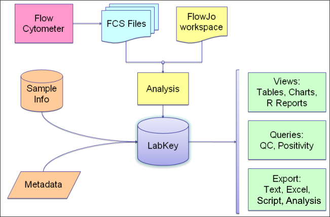
Analyses performed using FlowJo can be imported into LabKey where they can be refined, quality controlled, and integrated with other related data. The statistics calculated by FlowJo are read upon import from the workspace.
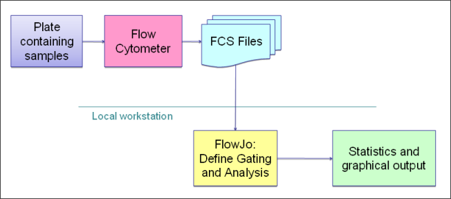
Graphs are generated for each sample and saved into the database. Note that graphs shown in LabKey are recreated from the Flow data using a different analysis engine than FlowJo uses. They are intended to give a rough 'gut check' of accuracy of the data and gating applied, but are not straight file copies of the graphs in FlowJo.

Annotate Flow Data Using Metadata, Keywords, and Background Information
Extra information can be linked to the run after the run has been imported via either LabKey Flow or FlowJo. Sample information uploaded from an Excel spreadsheet can also be joined to the well. Background wells can then be used to subtract background values from sample wells. Information on background wells is supplied through metadata.
The LabKey Flow Dashboard
You can use LabKey Server exclusively as a data repository and import results directly from a FlowJo workspace, or create an analysis script from a FlowJo workspace to apply to multiple runs. The dashboard will present relevant tasks and summaries.
LabKey Flow Module
The LabKey Flow module automates high-volume flow cytometry analysis. It is designed to manage large data sets from standardized assays spanning many instrument runs that share a common gating strategy.
To begin using LabKey Flow, an investigator first defines a gate template for an entire study using FlowJo, and uploads the FlowJo workspace to LabKey Server. He or she then points LabKey Flow to a repository of FCS files on a network file server, and starts an analysis.
LabKey Flow computes the compensation matrix, applies gates, calculates statistics, and generates graphs. Results are stored in a relational database and displayed using secure, interactive web pages.
Researchers can then define custom queries and views to analyze large result sets. Gate templates can be modified, and new analyses can be run and compared. Results can be printed, emailed, or exported to tools such as Excel or R for further analysis. LabKey Flow enables quality control and statistical positivity analysis over data sets that are too large to manage effectively using PC-based solutions.
Topics
- Flow Cytometry Overview
- Tutorial: Explore a Flow Workspace
- Tutorial: Set Flow Background
- Edit Keywords
- Add Sample Descriptions
- Add Statistics to FCS Queries
- Flow Module Schema
- Analysis Archive Format
Example Flow Usage Folders
FlowJo Version Notes
If you are using FlowJo version 10.8, you will need to upgrade to LabKey Server version 21.7.3 (or later) in order to properly handle "NaN" (Not a Number) in statistic values. Contact your Account Manager for details.
Additional Resources
Set Up a Flow Folder
Follow the steps in this topic to set up a "Flow Tutorial" folder. You will set up and import a basic workspace that you can use for two of the flow tutorials, listed at the bottom of this topic.
Create a Flow Folder
- Log in to your server and navigate to your "Tutorials" project. Create it if necessary.
- If you don't already have a server to work on where you can create projects, start here.
- If you don't know how to create projects and folders, review this topic.
- Create a new subfolder named "Flow Tutorial". Choose the folder type Flow.
Upload Data Files
- Click to download this "DemoFlow" archive. Unzip it.
- In the Flow Tutorial folder, under the Flow Summary section, click Upload and Import.
- Drag and drop the unzipped DemoFlow folder into the file browser. Wait for the sample files to be uploaded.
- When complete, you will see the files added to your project's file management system.
Import FlowJo Workspace
More details and options for importing workspaces are covered in the topic: Import a Flow Workspace and Analysis. To simply set up your environment for a tutorial, follow these steps:
- Click the Flow Tutorial link to return to the main folder page.
- Click Import FlowJo Workspace Analysis.
- Click Browse the pipeline and select DemoFlow > ADemoWorkspace.wsp as shown:
- Click Next.
Wizard Acceleration
When the files are in the same folder as the workspace file and all files are already associated with samples present in the workspace, you will skip the next two panels of the import wizard. If you need to adjust anything about either step, you can use the 'Back' option after the acceleration. Learn about completing these steps in this topic: Import a Flow Workspace and Analysis.
- On the Analysis Folder step, click Next to accept the defaults.
- Click Finish at the end of the wizard.
- Wait for the import to complete, during which you will see status messages.
When complete, you will see the workspace data.
- Click the Flow Tutorial link to return to the main folder page.
You are now set up to explore the Flow features and tutorials in your folder.
Related Topics
Tutorial: Explore a Flow Workspace
This tutorial teaches you how to:
- Set up a flow cytometry project
- Import flow data
- Create flow datasets
- Create reports based on your data
- Create quality control reports
Set Up
Tutorial Steps
- Step 1: Customize Your Grid View
- Step 2: Examine Graphs
- Step 3: Examine Well Details
- Step 4: Export Flow Data
- Step 5: Flow Quality Control
Related Topics
First Step
Step 1: Customize Your Grid View
The main Flow dashboard displays the following web parts by default:
- Flow Experiment Management: Links to perform actions like setting up an experiment and analyzing FCS files.
- Flow Summary: Common actions and configurations.
- Flow Analyses: Lists the flow analyses that have been performed in this folder.
- Flow Scripts: Lists analysis scripts. An analysis script stores the gating template definition, rules for calculating the compensation matrix, and the list of statistics and graphs to generate for an analysis.
Understanding Flow Column Names
In the flow workspace, statistics column names are of the form "subset:stat". For example, "Lv/L:%P" is used for the "Live Lymphocytes" subset and the "percent of parent" statistic.
Graphs are listed with parentheses and are of the form "subset(x-axis:y-axis)". For example, "Singlets(FSC-A:SSC-A)" for the "Singlets" subset showing forward and side scatter.
Customize Your Grid View
The columns displayed by default for a dataset are not necessarily the ones you are most interested in, so you can customize which columns are included in the default grid. See Customize Grid Views for general information about customizing grids.
In this first tutorial step, we'll show how you might remove one column, add another, and save this as the new default grid. This topic also explains the column naming used in this sample flow workspace.
- Begin on the main page of your Flow Tutorial folder.
- Click Analysis in the Flow Analyses web part.
- Click the Name: ADemoWorkspace.wsp.
- Select (Grid Views) > Customize Grid.
- This grid shows checkboxes for "Available Fields" (columns) in a panel on the left. The "Selected Fields" list on the right shows the checked fields.
- In the Selected Fields pane, hover over "Compensation Matrix". Notice that you see a tooltip with more information about the field and the (rename) and (remove) icons are activated.
- Click the to remove the field.
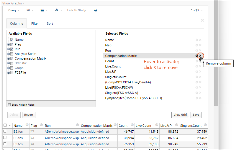
- In the Available Fields pane, open the Statistic node by clicking the icon (it will turn into a ) and click the checkbox for Singlets:%P to add it to the grid.
- By default, the new field will be listed after the field that was "active" before it was added - in this case "Count" which was immediately after the removed field. You can drag and drop the field elsewhere if desired.
- Before leaving the grid customizer, scroll down through the "Selected Fields" and notice some fields containing () parentheses. These are graph fields. You can also open the "Graph" node in the available fields panel and see they are checked.
- If you wanted to select all the graphs, for example, you could shift-click the checkbox for the top "Graph" node. For this tutorial, leave the default selections.
- Click Save.
- Confirm that Default grid view for this page is selected, and click Save.
You will now see the "Compensation Matrix" column is gone, and the "Singlets:%P" column is shown in the grid.
Notice that the graph columns listed as "selected" in the grid customizer are not shown as columns. The next step will cover displaying graphs.
Start Over | Next Step (2 of 5)
Step 2: Examine Graphs
In this step we will examine our data graphs. As you saw in the previous step, graphs are selected within the grid customizer but are not shown by default.
Review Graphs
- Return to the grid you customized (if you navigated away): from the Flow Tutorial page, in the Flow Analyses web part, click Analysis then ADemoWorkspace.wsp to return to the grid.
- Select Show Graphs > Inline.
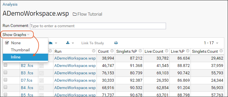
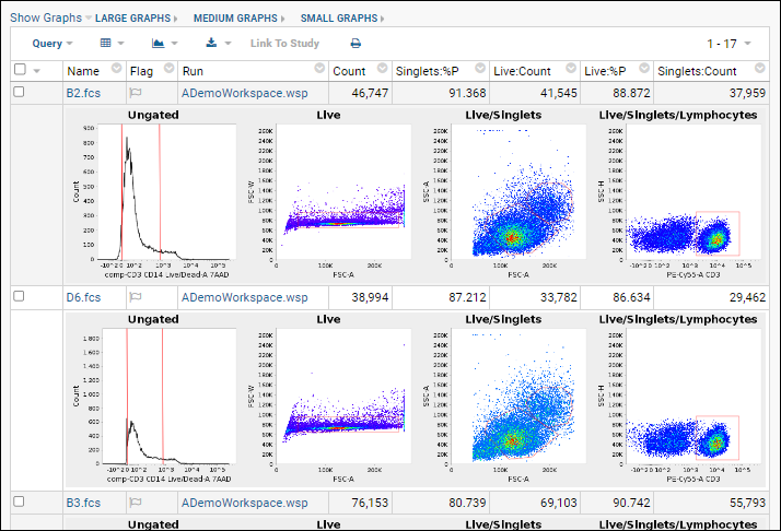
- The inline graphs are rendered. Remember we had selected 4 graphs; each row of the data grid now has an accompanying set of 4 graphs interleaved between them.
- Note: for large datasets, it may take some time for all graphs to render. Some metrics may not have graphs for every row.
- Three graph size options are available at the top of the data table. The default is medium.
- When viewing medium or small graphs, clicking on any graph image will show it in the large size.
- See thumbnail graphs in columns alongside other data by selecting Show Graphs > Thumbnail.
- Hovering over a thumbnail graph will pop forward the same large format as in the inline view.
- Hide graphs by selecting Show Graphs > None.
See a similar online example.
Review Other Information
The following pages provide other views and visualizations of the flow data.
- Scroll down to the bottom of the ADemoWorkspace.wsp page.
- Click Show Compensation to view the compensation matrix. In this example workspace, the graphs are not available, but you can see what compensated and uncompensated graphs would look like in a different dataset by clicking here.
- Go back in the browser.
- Click Experiment Run Graph and then choose the tab Graph Detail View to see a graphical version of this experiment run.
Previous Step | Next Step (3 of 5)
Step 3: Examine Well Details
Detailed statistics and graphs for each individual well can be accessed for any run. In this tutorial step, we review the details available.
Access Well Details
- Return to the flow dashboard in the Flow Tutorial folder.
- In the Flow Analyses web part, click Analysis then ADemoWorkspace.wsp to return to the grid.
- Hover over any row to reveal a (Details) link.
- Click it.
- The details view will look something like this:
You can see a similar online example here.
View More Graphs
- Scroll to the bottom of the page and click More Graphs.
- This allows you to construct additional graphs. You can choose the analysis script, compensation matrix, subset, and both axes.
- Click Show Graph to see the graph.
View Keywords from the FCS File
- Go back in your browser, or click the FCSAnalysis 'filename' link at the top of the Choose Graph page to return to the well details page.
- Click the name of the FCS File.
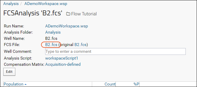
- Click the Keywords link to expand the list:
Previous Step | Next Step (4 of 5)
Step 4: Export Flow Data
Before you export your dataset, customize your grid to show the columns you want to export. For greater control of the columns included in a view, you can also create custom queries. Topics available to assist you:
After you have finalized your grid, you can export the displayed table to an Excel spreadsheet, a text file, a script, or as an analysis. Here we show an Excel export. Learn about exporting in an analysis archive in this topic:Export to Excel
- Return to the Flow Tutorial folder.
- Open the grid you have customized. In this tutorial, we made changes here in the first step.
- In the Flow Analyses web part, click Analysis.
- Click the Name: ADemoWorkspace.wsp.
- Click (Export).
- Choose the desired format using the tabs, then select options relevant to the format. For this tutorial example, select Excel (the default) and leave the default workbook selected.
- Click Export.
Note that export directly to Excel limits the number of rows. If you need to work around this limitation to export larger datasets, first export to a text file, then open the text file in Excel.
Related Topics
Previous Step | Next Step (5 of 5)
Step 5: Flow Quality Control
Quality control reports in the flow module can give you detailed insights into the statistics, data, and performance of your flow data, helping you to spot problems and find solutions. Monitoring controls within specified standard deviations can be done with Levey-Jennings plots. To generate a report:
- Click the Flow Tutorial link to return to the main folder page.
- Add a Flow Reports web part on the left.
- Click Create QC Report in the new Flow Reports web part.
- Provide a Name for the report, and select a Statistic.
- Choose whether to report on Count or Frequency of Parent.
- In the Filters box, you can filter the report by keyword, statistic, field, folder, and date.
- Click Save.
- The Flow Reports panel will list your report.
- Click the name to see the report. Use the manage link for the report to edit, copy, delete, or execute it.
The report displays results over time, followed by a Levey-Jennings plot with standard deviation guide marks. TSV format output is shown below the plots.
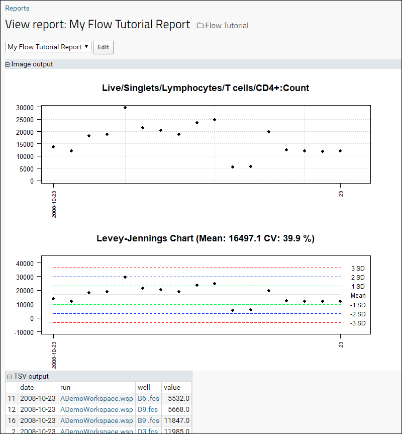
Congratulations
You have now completed the Tutorial: Explore a Flow Workspace. To explore more options using this same sample workspace, try this tutorial next:
Previous Step
Tutorial: Set Flow Background
If you have a flow cytometry experiment containing a background control (such as an unstimulated sample, an unstained sample, or a Fluorescence Minus One (FMO) control), you can set the background in LabKey for use in analysis. To perform this step we need to:
- Identify the background controls
- Associate the background values with their corresponding samples of interest
To gain familiarity with the basics of the flow dashboard, data grids, and using graphs, you can complete the Tutorial: Explore a Flow Workspace first. It uses the same setup and sample data as this tutorial.
Tutorial Steps:
- Set Up
- Upload Sample Descriptions
- Associate the Sample Descriptions with the FCS Files
- Add Keywords as Needed
- Set Metadata
- Use Background Information
- Flow Reports
Set Up
Upload Sample Descriptions
Sample descriptions give the flow module information about how to interpret a group of FCS files using keywords. The flow module uses a sample type named "Samples" which you must first define and structure correctly. By default it will be created at the project level, and thus shared with all other folders in the project, but there are several options for sharing sample definitions. Note that it is important not to rename this sample type. If you notice "missing" samples or are prompted to define it again, locate the originally created sample type and restore the "Samples" name.
Download these two files to use:
- Navigate to your Flow Tutorial folder. This is your flow dashboard.
- Click Upload Samples (under Manage in the Flow Summary web part).
- If you see the Import Data page, the sample type has already been defined and you can skip to the next section.
- On the Create Sample Type page, you cannot edit the name "Samples".
- In the Naming Pattern field, enter this string to use the "TubeName" column as the unique identifier for this sample type.
${TubeName} - You don't need to change other defaults here.
- Click the Fields section to open it.
- Click the for the Default System Fields to collapse the listing.
- Drag and drop the "Fields_FlowSampleDemo.fields.json" file into the target area for Custom Fields.
- You could instead click Manually Define Fields and manually add the fields.
- Ignore the blue banner asking if you want to add a unique ID field.
- Check that the fields added match the screencap below, and adjust names and types if not.
- Learn more about the field editor in this topic: Field Editor.
- Ignore any banner offering to add a unique ID field.
- Click Save.
- Return to the main dashboard by clicking the Flow Tutorial link near the top of the page.
You have now defined the sample type you need and will upload the actual sample information next.
Upload Samples
- In the Flow Tutorial folder, click Upload Samples.
- You can either copy/paste data as text or upload a file. For this tutorial, click Upload File.
- Leave the default Add samples selected.
- Click Browse to locate and select the "FlowSampleDemo.xlsx" file you downloaded.
- Do not check the checkbox for importing by alternate key.
- Click Submit.
Once it is uploaded, you will see the sample type.
Associate the Sample Descriptions with the FCS Files
- Return to the main dashboard by clicking the Flow Tutorial link near the top of the page.
- Click Define Sample Description Join Fields in the Flow Experiment Management web part.
- On the Join Samples page, set how the properties of the sample type should be mapped to the keywords in the FCS files.
- For this tutorial, select TubeName from the Sample Property menu, and Name from the FCS Property menu
- Click Update.
You will see how many FCS Files could be linked to samples. The number of files linked to samples may be different from the number of sample descriptions since multiple files can be linked to any given sample.
To see the grid of which samples were linked to which files:
- Click the Flow Tutorial link.
- Then click 17 sample descriptions (under "Assign additional meanings to keywords").
- Linked Samples and FCSFiles are shown first, with the values used to link them.
- Scroll down to see Unlinked Samples and Unlinked FCSFiles, if any.
Add Keywords as Needed
Keywords imported from FlowJo can be used to link samples, as shown above. If you want to add additional information within LabKey, you can do so using additional keywords.
- Return to the main Flow Tutorial dashboard.
- Click 17 FCS files under Import FCS Files.
- Select the rows to which you want to add a keyword and set a value. For this tutorial, click the box at the top of the column to select all rows.
- Click Edit Keywords.
- You will see the list of existing keywords.
- The blank boxes in the righthand column provide an opportunity to change the values of existing keywords. All selected rows would receive any value you assigned a keyword here. If you leave the boxes blank, no changes will be made to the existing data.
- For this tutorial, make no changes to the existing keyword values.
- Click Create a new keyword to add a new keyword for the selected rows.
- Enter "SampleType" as the keyword, and "Blood" as the value.
- Click Update.
- You will see the new SampleType column in the files data grid, with all (selected) rows set to "Blood".
If some of the samples were of another type, you could repeat the "Edit Keywords" process for the subset of rows of that other type, entering the same "SampleType" keyword and the alternate value.
Set Metadata
Setting metadata including participant and visit information for samples makes it possible to integrate flow data with other data about those participants.
Background and foreground match columns are used to identify the group -- using subject and timepoint is one option.
Background setting: it is used to identify which well or wells are background out of the group of wells. If more than one well is identified as background in the group, the background value will be averaged.
- Click the Flow Tutorial link near the top of the page to return to the main flow dashboard.
- Click Edit Metadata in the Flow Summary web part.
- On the Edit Metadata page, you can set three categories of metadata. Be sure to click Set Metadata at the bottom of the page when you are finished making changes.
- Sample Columns: Select how to identify your samples. There are two options:
- Set the Specimen ID column or
- Set the Participant column and set either a Visit column or Date column.
- Background and Foreground Match Columns
- Select the columns that match between both the foreground and background wells.
- You can select columns from the uploaded data, sample type, and keywords simultaneously as needed. Here we choose the participant ID since there is a distinct baseline for each participant we want to use.
- Background Column and Value
- Specify the column and how to filter the values to uniquely identify the background wells from the foreground wells.
- Here, we choose the "Sample WellType" column, and declare rows where the well type "Contains" "Baseline" as the background.
- When finished, click Set Metadata.
Use Background Information
- Click the Flow Tutorial link near the top of the page to return to the main flow dashboard.
- Click the Analysis Folder you want to view, here Analysis (1 run), in the Flow Summary web part.
- Click the name ADemoWorkspace.wsp to open the grid of workspace data.
- Select (Grid Views) > Customize Grid.
- Now you will see a node for Background.
- Click the icon to expand it.
- Use the checkboxes to control which columns are displayed.
- If they are not already checked, place checkmarks next to "BG Count", "BG Live:Count", "BG Live:%P", and "BG Singlets:Count".
- Click Save, then Save in the popup to save this grid view as the default.
Return to the view customizer to make the source of background data visible:
- Select (Grid Views) > Customize Grid.
- Expand the FCSFile node, then the Sample node, and check the boxes for "PTID" and "Well Type".
- Click View Grid.
- Click the header for PTID and select Sort Ascending.
- Click Save above the grid, then Save in the popup to save this grid view as the default.
- Now you can see that the data for each PTID's "Baseline" well is entered into the corresponding BG fields for all other wells for that participant.
Display graphs by selecting Show Graphs > Inline as shown here:
Congratulations
You have now completed the tutorial and can use this process with your own data to analyze data against your own defined background.
Import a Flow Workspace and Analysis
Once you have set up the folder and uploaded the FCS files, you can import a FlowJo workspace and then use LabKey Server to extract data and statistics of interest.
This topic uses a similar example workspace as in the Set Up a Flow Folder walkthrough, but includes intentional mismatches to demonstrate the full import wizard in more detail.
Import a FlowJo Workspace
- Click to download this "DemoFlowWizard" archive. Unzip it.
- In the Flow Tutorial folder, under the Flow Summary section, click Upload and Import.
- Click fileset in the left panel to ensure you are at the 'top' level of the file repository
- Drop the unzipped DemoFlowWizard folder into the target area to upload it.
- Click the Flow Tutorial link to return to the main folder page.
- Click Import FlowJo Workspace Analysis. This will start the process of importing the compensation and analysis (the calculated statistics) from a FlowJo workspace. The steps are numbered and the active step will be shown in bold.
- Select Browse the pipeline.
- In the left panel, click to expand the DemoFlowWizard folder.
- In the right panel, select the ADemoWorkspace.wsp file, and click Next.
Warnings
If any calculations are missing in your FlowJo workspace, you would see warnings at this point. They might look something like:Warnings (2):
Sample 118756.fcs (286): 118756.fcs: S/L/-: Count statistic missing
Sample 118756.fcs (286): 118756.fcs: S/L/FITC CD4+: Count statistic missing
The tutorial does not contain any such warnings, but if you did see them with your own data and needed to import these statistics, you would have to go back to FlowJo, re-calculate the missing statistics, and then save as xml again.
2. Select FCS Files If you completed the flow tutorial, you may have experienced an accelerated import wizard which skipped steps. If the wizard cannot be accelerated, you will see a message indicating the reason. In this case, the demo files package includes an additional file that is not included in the workspace file. You can proceed, or cancel and make adjustments if you expected a 1:1 match.
To proceed:
- If you have already imported the tutorial files into this folder, choose Previously imported FCS files in order to see the sample review process in the next step.
- If not, select Browse the pipeline for the directory of FCS files and check the box for the DemoFlowWizard folder.
- Click Next.
- The import wizard will attempt to match the imported samples from the FlowJo workspace with the FCS files. If you were importing samples that matched existing FCS files, such as reimporting a workspace, matched samples would have a green checkmark and unmatched samples would have a red checkmark. To manually correct any mistakes, select the appropriate FCS file from the combobox in the Matched FCS File column. See below for more on the exact algorithm used to resolve the FCS files.
- Confirm that all samples (= 17 samples) are selected and click Next.
- Accept the default name of your analysis folder, "Analysis". If you are analyzing the same set of files a second time, the default here will be "Analysis1".
- Click Next.
- Review the properties and click Finish to import the workspace.
- Wait for Import to Complete. While the job runs, you will see the current status file growing and have the opportunity to cancel if necessary. Import can take several minutes.
- When the import process completes, you will see a grid named "ADemoWorkspace.wsp" To learn how to customize this grid to display the columns of your choice, see this topic: Step 1: Customize Your Grid View.
Resolving FCS Files During Import
When importing analysis results from a FlowJo workspace or an external analysis archive, the Flow Module will attempt to find a previously imported FCS file to link the analysis results to.
The matching algorithm compares the imported sample from the FlowJo workspace or external analysis archive against previously imported FCS files using the following properties and keywords: FCS file name or FlowJo sample name, $FIL, GUID, $TOT, $PAR, $DATE, $ETIM. Each of the 7 comparisons are weighted equally. Currently, the minimum number of required matches is 2 -- for example, if only $FIL matches and others don't, there is no match.
While calculating the comparisons for each imported sample, the highest number of matching comparisons is remembered. Once complete, if there is only a single FCS file that has the max number of matching comparisons, it is considered a perfect match. The import wizard resolver step will automatically select the perfectly matching FCS file for the imported sample (they will have the green checkmark). As long as each FCS file can be uniquely matched by at least two comparisons (e.g., GUID and the other keywords), the import wizard should automatically select the correct FCS files that were previously imported.
If there are no exact matches, the imported sample will not be automatically selected (red X mark in the wizard) and the partially matching FCS files will be listed in the combo box ordered by number of matches.
Name Length Limitation
The names of Statistics and Graphs in the imported workspace cannot be longer than 400 characters. FlowJo may support longer names, but they cannot be imported into the LabKey Flow module. Names that exceed this limit will generate an import error similar to:
11 Jun 2021 16:51:21,656 ERROR: FlowJo Workspace import failed
org.labkey.api.query.RuntimeValidationException: name: Value is too long for column 'SomeName', a maximum length of 400 is allowed. Supplied value was 433 characters long.
Related Topics
Edit Keywords
Keywords imported from FlowJo can be used to link samples and provide metadata. This topic describes how you can edit the values assigned to those keywords and also add additional keywords within LabKey to store additional information.
Edit FCS Keyword Input Values
You can edit keyword input values either individually or in bulk.
- To edit existing FCS keywords, go to the FCS Files table and select one or more rows. Any changes made will be applied to all the selected rows.
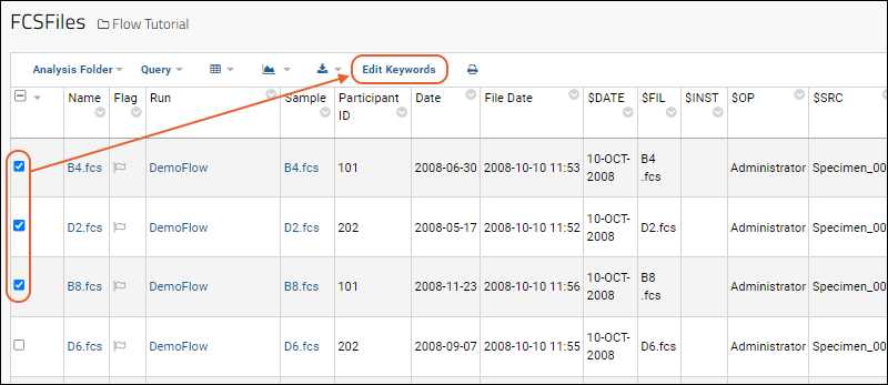
- Enter the new values for desired keywords in the blank text boxes provided.
- The FCS files to be changed are listed next to Selected Files.
- Existing values are not shown in the input form. Instead, a blank form is shown, even for keywords that have non-blank values.
- Click Update to submit the new values.
- If multiple FCS files are selected, the changes will be applied to them all.
- If an input value is left blank, no change will be made to the existing value(s) of that keyword for the selected rows.
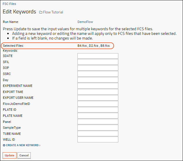
Add Keywords and Set Values
- To add a new keyword, click Create a New Keyword
- Enter the name of the keyword and a value for the selected rows. Both keyword and value are required.
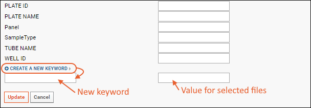
Note that if you want to add a new keyword for all rows, but set different values, you would perform multiple rounds of edits. First select all rows to add the new keyword, providing a default/common temporary value for all rows. Then select the subsets of rows with other values for that keyword and set a new value.
Display Keyword Values
New keywords are not always automatically shown in the data grid. To add the new keyword column to the grid:
- Select (Grid Views) > Customize Grid.
- In the Available Fields panel, open the node Keywords and select the new keyword.
- Click View Grid or Save to add it.
Related Topics
- Tutorial: Set Flow Background: This tutorial includes adding a new keyword.
Add Sample Descriptions
You can associate sample descriptions with flow data and associate sample columns with FCS keywords as described in this topic.
- Share "Samples" Sample Type
- Create "Samples" Sample Type
- Upload Sample Descriptions
- Define Sample Description Join Fields
- Add Sample Columns to View
Share "Samples" Sample Type
The flow module uses a sample type named "Samples". You cannot change this name expectation, and the type's properties and fields must be defined and available in your folder before you can upload or link to sample descriptions. Each folder container could have a different definition of the "Samples" sample type, or the definition could be shared at the project or site level.
For example, you might have a given set of samples and need to run a series of flow panels against the same samples in a series of subfolders. Or you might always have samples with the same properties across a site, though each project folder has a unique set of samples.
Site-wide Sharing
If you define a "Samples" sample type in the Shared project, you will be able to use the definition in any folder on the site. Each folder will have a distinct set of samples local to the container, i.e. any samples themselves defined in the Shared project will not be exposed in any local flow folder.
Follow the steps below to:
- Define the "Samples" sample type in the /Shared project. You do not need to add any samples to it.
- In each flow folder, you will bypass the definition step and be able to directly add your samples.
Project-wide Sharing
If you define a "Samples" sample type in the top level project, you will be able to use the definition in all subfolders of that project at any level. Each folder will also be able to share the samples defined in the project, i.e. you won't have to import sample descriptions into the local flow folder.
Follow the steps below to:
- Define the "Samples" sample type in the top-level project.
- Add the sample inventory at the project level.
- In each flow folder, you will bypass the definition step and can either:
- Add your samples to the local container, or
- Bypass adding new samples and link your new data to the project-level samples.
Create "Samples" Sample Type
To create a "Samples" sample type in a folder where it does not already exist (and where you do not want to share the definition), follow these steps.
- From the flow dashboard, click either Upload Sample Descriptions or Upload Samples.
- If you don't see the link for "Upload Sample Descriptions", and instead see "Upload More Samples", the sample type is already defined and you can proceed to uploading.
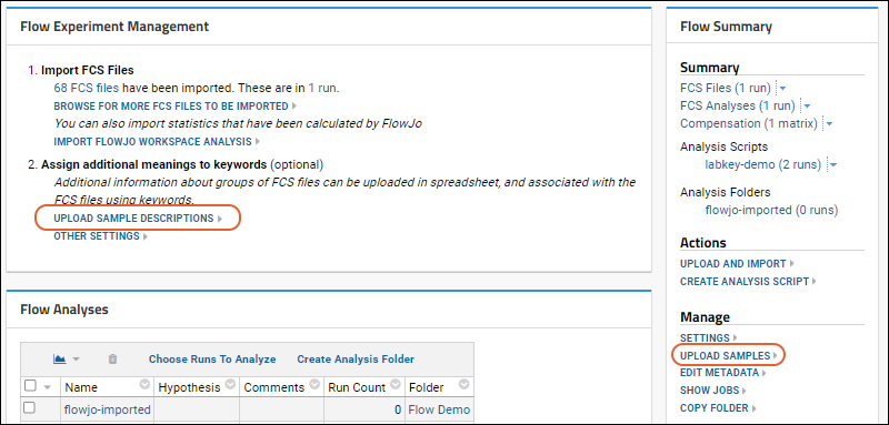
- On the Create Sample Type page, you cannot change the Name; it must be "Samples" in the flow module.
- You need to provide a unique way to identify the samples of this type.
- If your sample data contains a Name column, it will be used as the unique identifier.
- If not, you can provide a Naming Pattern for uniquely identifying the samples. For example, if you have a "TubeName" column, you can tell the server to use it by making the Naming Pattern "${TubeName}" as shown here:
- Click the Fields section to open it.
- Review the Default System Fields.
- Fields with active checkboxes in the Enabled column can be 'disabled' by unchecking the box.
- The Name of a sample is always required, and you can check the Required boxes to make other fields mandatory.
- Collapse this section by clicking the . It will become a .
- You have several options for defining Custom Fields for your samples:
- Import or infer fields from file: Drag and drop or select a file to use for defining fields:
- Infer from a data spreadsheet. Supported formats include: .csv, .tsv, .txt, .xls, and .xlsx.
- Or import field definitions from a prepared JSON file. For example, this JSON file will create the fields shown below: Fields_FlowSampleDemo.fields.json
- Manually Define Fields: Click and use the field editor to add new fields.
- Learn more about defining sample type fields in this topic: Create Sample Type.
- See an example using the following fields in this tutorial: Tutorial: Set Flow Background.
When finished, click Save to create the sample type.
You will return to the main dashboard where the link Upload Sample Descriptions now reads Upload More Samples.
Upload Sample Descriptions
- Once the "Samples" sample type is defined, clicking Upload Samples (or Upload More Samples) will open the panel for importing your sample data.
- Click Download Template to download a template showing all the necessary columns for your sample type.
- You have two upload options:
- Either Copy/Paste data into the Data box shown by default, and select the appropriate Format: (TSV or CSV). The first row must contain column names.
- OR
- Click Upload file (.xlsx, .xls, .csv, .txt) to open the file selection panel, browse to your spreadsheet and open it. For our field definitions, you can use this spreadsheet: FlowSampleDemo.xlsx
- Import Options: The default selection is Add Samples, i.e. fail if any provided samples already defined.
- Change the selection if you want to Update samples, and check the box if you also want to Allow new samples during update, otherwise, new samples will cause import to fail.
- For either option, choose whether to Import Lookups by Alternate Key.
- Click Submit.
Define Sample Description Join Fields
Once the samples are defined, either by uploading locally, or at the project-level, you can associate the samples with FCS files using one or more sample join fields. These are properties of the sample that need to match keywords of the FCS files.
- Click Flow Tutorial (or other name of your folder) to return to the flow dashboard.
- Click Define sample description join fields and specify the join fields. Once fields are specified, the link will read "Modify sample description join fields". For example:
| Sample Property | FCS Property |
|---|---|
| "TubeName" | "Name" |
- Click Update.
Return to the flow dashboard and click the link ## sample descriptions (under "Assign additional meanings to keywords"). You will see which Samples and FCSFiles could be linked, as well as the values used to link them.
Scroll down for sections of unlinked samples and/or files, if any. Reviewing the values for any entries here can help troubleshoot any unexpected failures to link and identify the right join fields to use.
Add Sample Columns to View
You will now see a new Sample column in the FCSFile table and can add it to your view:
- Click Flow Tutorial (or other name of your folder).
- Click FCS Files in the Flow Summary on the right.
- Click the name of your files folder (such as DemoFlow).
- Select (Grid Views) > Customize Grid.
- Expand the Sample node to see the columns from this table that you may add to your grid.
Related Topics:
Add Statistics to FCS Queries
This topic covers information helpful in writing some flow-specific queries. Users who are new to custom queries should start with this section of the documentation:
LabKey SQL provides the "Statistic" method on FCS tables to allow calculation of certain statistics for FCS data.- Example: StatisticDemo Query - Use the SQL Designer to add/remove "Statistic" fields to a FCS query.
- Example: SubsetDemo Query - Calculate suites of statistics for every well.
Example: StatisticDemo Query
For this example, we create a query called "StatisticDemo" based on the FCSAnalyses dataset. Start from your Flow demo folder, such as that created during the Flow Tutorial.
Create a New Query
- Select > Go To Module > Query.
- Click flow to open the flow schema.
- Click Create New Query.
- Call your new query "StatisticDemo"
- Select FCSAnalyses as the base for your new query.
- Click Create and Edit Source.
Add Statistics to the Generated SQL
The default SQL simply selects all the columns:
SELECT FCSAnalyses.Name,
  FCSAnalyses.Flag,
  FCSAnalyses.Run,
  FCSAnalyses.CompensationMatrix
FROM FCSAnalyses
- Add a line to include the 'Count' statistic like this. Remember to add the comma to the prior line.
SELECT FCSAnalyses.Name,
  FCSAnalyses.Flag,
  FCSAnalyses.Run,
  FCSAnalyses.CompensationMatrix,
  FCSAnalyses.Statistic."Count"
FROM FCSAnalyses
- Click Save.
- Click the Data tab. The "Count" statistic has been calculated using the Statistic method on the FCSAnalyses table, and is shown on the right.
You can flip back and forth between the source, data, and xml metadata for this query using the tabs in the query editor.
Run the Query
From the "Source" tab, to see the generated query, either view the "Data" tab, or click Execute Query. To leave the query editor, click Save & Finish.
The resulting table includes the "Count" column on the right:
View this query applied to a more complex dataset. The dataset used in the Flow Tutorial has been slimmed down for ease of use. A larger, more complex dataset can be seen in this table:
Example: SubsetDemo Query
It is possible to calculate a suite of statistics for every well in an FCS file using an INNER JOIN technique in conjunction with the "Statistic" method. This technique can be complex, so we present an example to provide an introduction to what is possible.
Create a Query
For this example, we use the FCSAnalyses table in the Peptide Validation Demo. We create a query called "SubsetDemo" using the "FCSAnalyses" table in the "flow" schema and edit it in the SQL Source Editor.
SELECT
  FCSAnalyses.FCSFile.Run AS ASSAYID,
  FCSAnalyses.FCSFile.Sample AS Sample,
  FCSAnalyses.FCSFile.Sample.Property.PTID,
  FCSAnalyses.FCSFile.Keyword."WELL ID" AS WELL_ID,
  FCSAnalyses.Statistic."Count" AS COLLECTCT,
  FCSAnalyses.Statistic."S:Count" AS SINGLETCT,
  FCSAnalyses.Statistic."S/Lv:Count" AS LIVECT,
  FCSAnalyses.Statistic."S/Lv/L:Count" AS LYMPHCT,
  FCSAnalyses.Statistic."S/Lv/L/3+:Count" AS CD3CT,
  Subsets.TCELLSUB,
  FCSAnalyses.Statistic(Subsets.STAT_TCELLSUB) AS NSUB,
  FCSAnalyses.FCSFile.Keyword.Stim AS ANTIGEN,
  Subsets.CYTOKINE,
  FCSAnalyses.Statistic(Subsets.STAT_CYTNUM) AS CYTNUM,
FROM FCSAnalyses
INNER JOIN lists.ICS3Cytokine AS Subsets ON Subsets.PFD IS NOT NULL
WHERE FCSAnalyses.FCSFile.Keyword."Sample Order" NOT IN ('PBS','Comp')
Examine the Query
This SQL code leverages the FCSAnalyses table and a list of desired statistics to calculate those statistics for every well.
The "Subsets" table in this query comes from a user-created list called "ICS3Cytokine" in the Flow Demo. It contains the group of statistics we wish to calculate for every well.
View Results
Results are available in this table.
Related Topics
Flow Module Schema
LabKey modules expose their data to the LabKey query engine in one or more schemas. This reference topic outlines the schema used by the Flow module to assist you when writing custom Flow queries.
Flow Module
The Flow schema has the following tables in it:
Runs Table | |
| This table shows experiment runs for all three of the Flow protocol steps. It has the following columns: | |
| RowId | A unique identifier for the run. Also, when this column is used in a query, it is a lookup back to the same row in the Runs table. That is, including this column in a query will allow the user to display columns from the Runs table that have not been explicitly SELECTed into the query |
| Flag | The flag column. It is displayed as an icon which the user can use to add a comment to this run. The flag column is a lookup to a table which has a text column “comment”. The icon appears different depending on whether the comment is null. |
| Name | The name of the run. In flow, the name of the run is always the name of the directory which the FCS files were found in. |
| Created | The date that this run was created. |
| CreatedBy | The user who created this run. |
| Folder | The folder or project in which this run is stored. |
| FilePathRoot | (hidden) The directory on the server's file system where this run's data files come from. |
| LSID | The life sciences identifier for this run. |
| ProtocolStep | The flow protocol step of this run. One of “keywords”, “compensation”, or “analysis” |
| RunGroups | A unique ID for this run. |
| AnalysisScript | The AnalysisScript that was used in this run. It is a lookup to the AnalysisScripts table. It will be null if the protocol step is “keywords” |
| Workspace | |
| CompensationMatrix | The compensation matrix that was used in this run. It is a lookup to the CompensationMatrices table. |
| TargetStudy | |
| WellCount | The number of FCSFiles that we either inputs or outputs of this run. |
| FCSFileCount | |
| CompensationControlCount | |
| FCSAnalysisCount | |
CompensationMatrices Table | |
| This table shows all of the compensation matrices that have either been calculated in a compensation protocol step, or uploaded. It has the following columns in it: | |
| RowId | A unique identifier for the compensation matrix. |
| Name | The name of the compensation matrix. Compensation matrices have the same name as the run which created them. Uploaded compensation matrices have a user-assigned name. |
| Flag | A flag column to allow the user to add a comment to this compensation matrix |
| Created | The date the compensation matrix was created or uploaded. |
| Protocol | (hidden) The protocol that was used to create this compensation matrix. This will be null for uploaded compensation matrices. For calculated compensation matrices, it will be the child protocol “Compensation” |
| Run | The run which created this compensation matrix. This will be null for uploaded compensation matrices. |
| Value | A column set with the values of compensation matrix. Compensation matrix values have names which are of the form “spill(channel1:channel2)” |
In addition, the CompensationMatrices table defines a method Value which returns the corresponding spill value.
The following are equivalent:
CompensationMatrices.Value."spill(FL-1:FL-2) "
CompensationMatrices.Value('spill(FL-1:FL-2)')
The Value method would be used when the name of the statistic is not known when the QueryDefinition is created, but is found in some other place (such as a table with a list of spill values that should be displayed).
FCSFiles Table | |
| The FCSFiles table lists all of the FCS files in the folder. It has the following columns: | |
| RowId | A unique identifier for the FCS file |
| Name | The name of the FCS file in the file system. |
| Flag | A flag column for the user to add a comment to this FCS file on the server. |
| Created | The date that this FCS file was loaded onto the server. This is unrelated to the date of the FCS file in the file system. |
| Protocol | (hidden) The protocol step that created this FCS file. It will always be the Keywords child protocol. |
| Run | The experiment run that this FCS file belongs to. It is a lookup to the Runs table. |
| Keyword | A column set for the keyword values. Keyword names are case sensitive. Keywords which are not present are null. |
| Sample | The sample description which is linked to this FCS file. If the user has not uploaded sample descriptions (i.e. defined the target table), this column will be hidden. This column is a lookup to the samples.Samples table. |
In addition, the FCSFiles table defines a method Keyword which can be used to return a keyword value where the keyword name is determined at runtime.
FCSAnalyses Table | |
| The FCSAnalyses table lists all of the analyses of FCS files. It has the following columns: | |
| RowId | A unique identifier for the FCSAnalysis |
| Name | The name of the FCSAnalysis. The name of an FCSAnalysis defaults to the same name as the FCSFile. This is a setting which may be changed. |
| Flag | A flag column for the user to add a comment to this FCSAnalysis. |
| Created | The date that this FCSAnalysis was created. |
| Protocol | (hidden) The protocol step that created this FCSAnalysis. It will always be the Analysis child protocol. |
| Run | The run that this FCSAnalysis belongs to. Note that FCSAnalyses.Run and FCSAnalyses.FCSFile.Run refer to different runs. |
| Statistic | A column set for statistics that were calculated for this FCSAnalysis. |
| Graph | A column set for graphs that were generated for this FCSAnalysis. Graph columns display nicely on LabKey, but their underlying value is not interesting. They are a lookup where the display field is the name of the graph if the graph exists, or null if the graph does not exist. |
| FCSFile | The FCSFile that this FCSAnalysis was performed on. This is a lookup to the FCSFiles table. |
In addition, the FCSAnalyses table defines the methods Graph, and Statistic.
CompensationControls Table | |||||||
| The CompensationControls table lists the analyses of the FCS files that were used to calculate compensation matrices. Often (as in the case of a universal negative) multiple CompensationControls are created for a single FCS file. The CompensationControls table has the following columns in it: | |||||||
| RowId | A unique identifier for the compensation control | ||||||
| Name | The name of the compensation control. This is the channel that it was used for, followed by either “+”, or “-“ | ||||||
| Flag | A flag column for the user to add a comment to this compensation control. | ||||||
| Created | The date that this compensation control was created. | ||||||
| Protocol | (hidden) | ||||||
| Run | The run that this compensation control belongs to. This is the run for the compensation calculation, not the run that the FCS file belongs to. | ||||||
| Statistic | A column set for statistics that were calculated for this compensation control. The following statistics are calculated for a compensation control:
|
||||||
| Graph | A column set for graphs that were generated for this compensation control. The names of graphs for compensation controls are of the form:
comp(channelName) or comp(<channelName>) The latter is shows the post-compensation graph. |
||||||
In addition, the CompensationControls table defines the methods Statistic and Graph.
AnalysisScripts Table | |
| The AnalysisScripts table lists the analysis scripts in the folder. This table has the following columns: | |
| RowId | A unique identifier for this analysis script. |
| Name | The user-assigned name of this analysis script |
| Flag | A flag column for the user to add a comment to this analysis script. |
| Created | The date this analysis script was created. |
| Protocol | (hidden) |
| Run | (hidden) |
Analyses Table | |
| The Analyses table lists the experiments in the folder with the exception of the one named Flow Experiment Runs. This table has the following columns: | |
| RowId | A unique identifier |
| LSID | (hidden) |
| Name | |
| Hypothesis | |
| Comments | |
| Created | |
| CreatedBy | |
| Modified | |
| ModifiedBy | |
| Container | |
| CompensationRunCount | The number of compensation calculations in this analysis. It is displayed as a hyperlink to the list of compensation runs. |
| AnalysisRunCount | The number of runs that have been analyzed in this analysis. It is displayed as a hyperlink to the list of those run analyses |
Analysis Archive Format
The LabKey flow module supports importing and exporting analyses as a series of .tsv and supporting files in a zip archive. The format is intended to be simple for tools to reformat the results of an external analysis engine for importing into LabKey. Notably, the analysis definition is not included in the archive, but may be defined elsewhere in a FlowJo workspace gating hierarchy, an R flowCore script, or be defined by some other software package.
Export an Analysis Archive
From the flow Runs or FCSAnalysis grid, you can export the analysis results including the original FCS files, keywords, compensation matrices, and statistics.
- Open the analysis and select the runs to export.
- Select (Export).
- Click the Analysis tab.
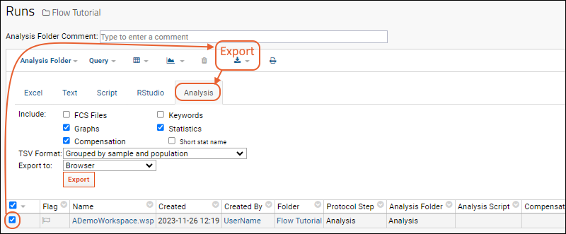
- Make the selections you need and click Export.
Import an Analysis Archive
To import a flow analysis archive, perhaps after making changes outside the server to add different statistics, graphs, or other information, follow these steps:
- In the flow folder, Flow Summary web part, click Upload and Import.
- Drag and drop the analysis archive into the upload panel.
- Select the archive and click Import Data.
- In the popup, confirm that Import External Analysis is selected.
- Click Import.
Analysis Archive Format
In brief, the archive format contains the following files:
 <root directory>
 ├─ keywords.tsv
 ├─ statistics.tsv
 │
 ├─ compensation.tsv
 ├─ <comp-matrix01>
 ├─ <comp-matrix02>.xml
 │
 ├─ graphs.tsv
 │
 ├─ <Sample Name 01>/
 │  └─ <graph01>.png
 │  └─ <graph02>.svg
 │
 └─ <Sample Name 02>/
    ├─ <graph01>.png
    └─ <graph02>.pdf
All analysis tsv files are optional. The keywords.tsv file lists the keywords for each sample. The statistics.tsv file contains summary statistic values for each sample in the analysis grouped by population. The graphs.tsv contains a catalog of graph images for each sample where the image format may be any image format (pdf, png, svg, etc.) The compensation.tsv contains a catalog of compensation matrices. To keep the directory listing clean, the graphs or compensation matrices may be grouped into sub-directories. For example, the graph images for each sample could be placed into a directory with the same name as the sample.
ACS Container Format
The ACS container format is not sufficient for direct import to LabKey. The ACS table of contents only includes relationships between files and doesn’t include, for example, the population name and channel/parameter used to calculate a statistic or render a graph. If the ACS ToC could include those missing metadata, the graphs.tsv would be made redundant. The statistics.tsv would still be needed, however.
If you have analyzed results tsv files bundled inside an ACS container, you may be able to extract portions of the files for reformatting into the LabKey flow analysis archive zip format, but you would need to generate the graphs.tsv file manually.
Statistics File
The statistics.tsv file is a tab-separated list of values containing stat names and values. The statistic values may be grouped in a few different ways: (a) no grouping (one statistic value per line), (b) grouped by sample (each column is a new statistic), (c) grouped by sample and population (the current default encoding), or (d) grouped by sample, population, and channel.Sample Name
Samples are identified by the value in the sample column so must be unique in the analysis. Usually the sample name is just the FCS file name including the ‘.fcs’ extension (e.g., “12345.fcs”).Population Name
The population column is a unique name within the analysis that identifies the set of events that the statistics were calculated from. A common way to identify the statistics is to use the gating path with gate names separated by a forward slash. If the population name starts with “(” or contains one of “/”, “{”, or “}” the population name must be escaped. To escape illegal characters, wrap the entire gate name in curly brackets { }. For example, the population “A/{B/C}” is the sub-population “B/C” of population “A”.Statistic Name
The statistic is encoded in the column header as statistic(parameter:percentile) where the parameter and percentile portions are required depending upon the statistic type. The statistic part of the column header may be either the short name (“%P”) or the long name (“Frequency_Of_Parent”). The parameter part is required for the frequency of ancestor statistic and for other channel based statistics. The frequency of ancestor statistic uses the name of an ancestor population as the parameter value while the other statistics use a channel name as the parameter value. To represent compensated parameters, the channel name is wrapped in angle brackets, e.g “<FITC-A>”. The percentile part is required only by the “Percentile” statistic and is an integer in the range of 1-99.The statistic value is a either an integer number or a double. Count stats are integer values >= 0. Percentage stats are doubles in the range 0-100. Other stats are doubles. If the statistic is not present for the given sample and population, it is left blank.
Allowed Statistics
| Short Name | Long Name | Parameter | Type |
|---|---|---|---|
| Count | Count | n/a | Integer |
| % | Frequency | n/a | Double (0-100) |
| %P | Frequency_Of_Parent | n/a | Double (0-100) |
| %G | Frequency_Of_Grandparent | n/a | Double (0-100) |
| %of | Frequency_Of_Ancestor | ancestor population name | Double (0-100) |
| Min | Min | channel name | Double |
| Max | Max | channel name | Double |
| Median | Median | channel name | Double |
| Mean | Mean | channel name | Double |
| GeomMean | Geometric_Mean | channel name | Double |
| StdDev | Std_Dev | channel name | Double |
| rStdDev | Robust_Std_Dev | channel name | Double |
| MAD | Median_Abs_Dev | channel name | Double |
| MAD% | Median_Abs_Dev_Percent | channel name | Double (0-100) |
| CV | CV | channel name | Double |
| rCV | Robust_CV | channel name | Double |
| %ile | Percentile | channel name and percentile 1-99 | Double (0-100) |
For example, the following are valid statistic names:
- Count
- Robust_CV(<FITC>)
- %ile(<Pacific-Blue>:30)
- %of(Lymphocytes)
Examples
NOTE: The following examples are for illustration purposes only.
No Grouping: One Row Per Sample and Statistic
The required columns are Sample, Population, Statistic, and Value. No extra columns are present. Each statistic is on a new line.| Sample | Population | Statistic | Value |
|---|---|---|---|
| Sample1.fcs | S/L/Lv/3+/4+/IFNg+IL2+ | %P | 0.85 |
| Sample1.fcs | S/L/Lv/3+/4+/IFNg+IL2- | Count | 12001 |
| Sample2.fcs | S/L/Lv/3+/{escaped/slash} | Median(FITC-A) | 23,000 |
| Sample2.fcs | S/L/Lv/3+/4+/IFNg+IL2+ | %ile(<Pacific-Blue>:30) | 0.93 |
Grouped By Sample
The only required column is Sample. The remaining columns are statistic columns where the column name contain the population name and statistic name separated by a colon.| Sample | S/L/Lv/3+/4+/IFNg+IL2+:Count | S/L/Lv/3+/4+/IFNg+IL2+:%P | S/L/Lv/3+/4+/IFNg+IL2-:%ile(<Pacific-Blue>:30) | S/L/Lv/3+/4+/IFNg+IL2-:%P |
|---|---|---|---|---|
| Sample1.fcs | 12001 | 0.93 | 12314 | 0.24 |
| Sample2.fcs | 13056 | 0.85 | 13023 | 0.56 |
Grouped By Sample and Population
The required columns are Sample and Population. The remaining columns are statistic names including any required parameter part and percentile part.| Sample | Population | Count | %P | Median(FITC-A) | %ile(<Pacific-Blue>:30) |
|---|---|---|---|---|---|
| Sample1.fcs | S/L/Lv/3+/4+/IFNg+IL2+ | 12001 | 0.93 | 45223 | 12314 |
| Sample1.fcs | S/L/Lv/3+/4+/IFNg+IL2- | 12312 | 0.94 | 12345 | |
| Sample2.fcs | S/L/Lv/3+/4+/IFNg+IL2+ | 13056 | 0.85 | 13023 | |
| Sample2.fcs | S/L/Lv/{slash/escaped} | 3042 | 0.35 | 13023 |
Grouped By Sample, Population, and Parameter
The required columns are Sample, Population, and Parameter. The remaining columns are statistic names with any required percentile part.| Sample | Population | Parameter | Count | %P | Median | %ile(30) |
|---|---|---|---|---|---|---|
| Sample1.fcs | S/L/Lv/3+/4+/IFNg+IL2+ | 12001 | 0.93 | |||
| Sample1.fcs | S/L/Lv/3+/4+/IFNg+IL2+ | FITC-A | 45223 | |||
| Sample1.fcs | S/L/Lv/3+/4+/IFNg+IL2+ | <Pacific-Blue> | 12314 |
Graphs File
The graphs.tsv file is a catalog of plot images generated by the analysis. It is similar to the statistics file and lists the sample name, plot file name, and plot parameters. Currently, the only plot parameters included in the graphs.tsv are the population and x and y axes. The graph.tsv file contains one graph image per row. The population column is encoded in the same manner as in the statistics.tsv file. The graph column is the colon-concatenated x and y axes used to render the plot. Compensated parameters are surrounded with <> angle brackets. (Future formats may split x and y axes into separate columns to ease parsing.) The path is a relative file path to the image (no “.” or “..” is allowed in the path) and the image name is usually just an MD5-sum of the graph bytes.
Multi-sample or multi-plot images are not yet supported.
| Sample | Population | Graph | Path |
|---|---|---|---|
| Sample1.fcs | S/L/Lv/3+/4+/IFNg+IL2+ | <APC-A> | sample01/graph01.png |
| Sample1.fcs | S/L/Lv/3+/4+/IFNg+IL2- | SSC-A:<APC-A> | sample01/graph02.png |
| Sample2.fcs | S/L/Lv/3+/4+/IFNg+IL2+ | FSC-H:FSC-A | sample02/graph01.svg |
| ... |
Compensation File
The compensation.tsv file maps sample names to compensation matrix file paths. The required columns are Sample and Path. The path is a relative file path to the matrix (no “.” or “..” is allowed in the path). The comp. matrix file is in the FlowJo comp matrix file format or a GatingML transforms:spilloverMatrix XML document.| Sample | Path |
|---|---|
| Sample1.fcs | compensation/matrix1 |
| Sample2.fcs | compensation/matrix2.xml |
Keywords File
The keywords.tsv lists the keyword names and values for each sample. This file has the required columns Sample, Keyword, and Value.| Sample | Keyword | Value |
|---|---|---|
| Sample1.fcs | $MODE | L |
| Sample1.fcs | $DATATYPE | F |
| ... |
Add Flow Data to a Study
For Flow data to be added to a study, it must include participant/timepoint ids or specimen ids, which LabKey Server uses to align the data into a structured, longitudinal study. The topic below describes four available mechanisms for supplying these ids to Flow data.
- Add Keywords Before Import to LabKey
- Add Keywords After Import to LabKey
- Associate Metadata Using a Sample Type
- Add Participant/Visit Data during the Link-to-Study Process
1. Add Keywords Before Import to LabKey
Add keywords to the flow data before importing them into LabKey. If your flow data already has keywords for either the SpecimenId or for ParticipantId and Timepoints, then you can link the Flow data into a study without further modification.
You can add keywords to an FCS file in most acquisition software, such as FlowJo. You can also add keywords in the WSP file, which LabKey will pick up. Use this method when you have control over the Flow source files, and if it is convenient to change them before import.
2. Add Keywords After Import to LabKey
If your flow data does not already contain the appropriate keywords, you can add them after import to LabKey Server. Note this method does not change the original FCS or WSP files. The additional keyword data only resides inside LabKey Server. Use this method when you cannot change the source Flow files, or when it is undesirable to do so.
- Navigate to the imported FCS files.
- Select one or more files from the grid. The group of files you select should apply to one participant.
- Click Edit Keywords.
- Scroll down to the bottom of the page and click Create a New Keyword.
- Add keywords appropriate for your target study. There are three options:
- Add a SpecimenId field (if you have a Specimen Repository in your study).
- Add a ParticipantId field and a Visit field (if you have a visit-based study without a Specimen Repository).
- Add a ParticipantId field and a Data field (if you have a based-based study without a Specimen Repository).
- Add values.
- Repeat for each participant in your study.
- Now your FCS files are linked to participants, and are ready for addition to a study.
3. Associate Metadata Using a Sample Type
This method extends the information about the flow samples to include participant ids, visits, etc. It uses a sample type as a mapping table, associating participant/visit metadata with the flow vials.
For example, if you had Flow data like the following:
| TubeName | PLATE_ID | FlowJoFileID | and so on... |
|---|---|---|---|
| B1 | 123 | 4110886493 | ... |
| B2 | 345 | 3946880114 | ... |
| B3 | 789 | 8693541319 | ... |
You could extend the fields with a sample type like
| TubeName | PTID | Date | Visit |
|---|---|---|---|
| B1 | 202 | 2009-01-18 | 3 |
| B2 | 202 | 2008-11-23 | 2 |
| B3 | 202 | 2008-10-04 | 1 |
- Add a sample type that contains the ptid/visit data.
- Under Manage, click Upload Samples.
- For an example see: Upload Sample Descriptions.
- Associate the sample type with the flow data (FCS files).
- Under Assign additional meanings to keywords, click Define/Modify Sample Description Join Fields.
- On the left select the vial name in the flow data; on the right select vial name in the sample type. This extends the descriptions of the flow vials to include the fields in the sample type.
- For an example see: Associate the Sample Type Descriptions with the FCS Files.
- Map to the Study Fields.
- Under Manage, click Edit Metadata.
- For an example, Set Metadata.
- To view the extended descriptions: Under Analysis Folders, click the analysis you want to link to a study. Click the run you wish to link. You may need to use (Grid Views) > Customize Grid to add the ptid/visit fields.
- To link to study: select from the grid and click Link to Study.
4. Add Participant/Visit Data During the Link-to-Study Process
You can manually add participant/visit data as part of the link-to-study wizard. For details see Link Assay Data into a Study.
Related Topics
FCS keyword utility
The keywords.jar file attached to this page is a simple commandline tool to dump the keywords from a set of FCS files. Used together with findstr or grep this can be used to search a directory of fcs files.
Download the jar file: keywords.jar
The following will show you all the 'interesting' keywords from all the files in the current directory (most of the $ keywords are hidden).
java -jar keywords.jar *.fcs
The following will show the EXPERIMENT ID, Stim, and $Tot keywords for each fcs file. You may need to escape the '$' on linux command line shells.
java -jar keywords.jar -k "EXPERIMENT ID,Stim,$Tot" *.fcsFor tabular output suitable for import into excel or other tools, use the "-t" switch:
java -jar keywords.jar -t -k "EXPERIMENT ID,Stim,$Tot" *.fcsTo see a list of all options:
java -jar keywords.jar --help